Материал: искусственный интеллект

J.B. Broekaert, et al. Cognitive Psychology 117 (2020) 101262

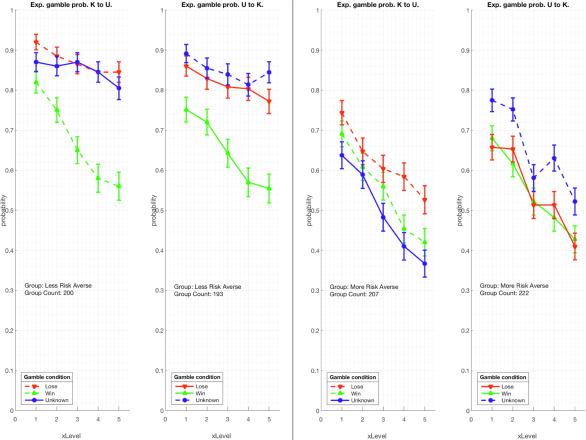
From Fig. S3, we observe that a substantial fraction of the participants obtained a single-gamble score of 10. Participants that always take the initial gamble, regardless the payoff, can be considered more risk-seeking than participants that will not always take it. This criterion warrants a partitioning of the sample by either obtaining a single-gamble score less than 10 or the maximum of 10, resulting in a ‘More risk averse’ group (N = 429) and a ‘Less risk averse’ group (N = 393) which are approximately of the same size.7 A first overall observation of the second-stage gamble probabilities separated along our criterion for risk attitude, Fig. 4 confirms some basic expectations. The defined ‘More risk averse’ group is indeed more risk averse than the defined ‘Less risk averse’ group, since all gamble probabilities for all payoff values X and for all outcome conditions are lower in the ‘More risk averse’ group in comparison to the same gambles taken by the ‘Less risk averse’ group. Moreover, the ‘More risk averse’ participants have a faster diminishing motivation to take the second-stage gamble for increasing payoff X when the first-stage gamble outcome was Lose or Unknown. However, when the first-stage gamble outcome was Win, this diminishing motivation to gamble over X remains the same for both groups. The ‘Less risk averse’ participants also show a significant distinction between gamble choices under W and L condition, while the ‘More risk averse’ participants hardly discriminate between these two conditions.8

A major and rather surprising observation for the ‘More risk averse’ group is the strong flow-order with outcome-condition crossover interaction (Fig. 4, right panel). Remarkably the ‘More risk averse’ participants show a tendency for a Disjunction Effect in K-to- U order and a significant inflative violation of the LTP in U-to-K order. Notice that this is a between-participants effect of flow order. A mixed ANOVA with unbalanced design (N = 207/N = 222) and with a dependent variable gamble probabilities (averaged across all payoffs X) and independent variables first-stage gamble outcome condition {W, L, U} and order {‘K-to-U’, ‘U-to-K’} revealed a significant interaction, F (2, 1281) = 12.78, p = 3. 20e 06 .

By contrast, there were no main effects for either first-gamble outcome condition or order in the ‘More risk averse’ group. That is, surprisingly, there appears to be no effect on choice behavior from whether the first-stage gamble was indicated as Won or Lost.

The ‘Less risk averse’ participants do not show any tendency for a Disjunction Effect in the order K-to-U, while in the U-to-K order a non-significant tendency for an inflative violation of the LTP occurs. A mixed ANOVA with unbalanced design (N = 200/N = 193), testing for factors of condition {W, L, U} and order {‘K-to-U’, ‘U-to-K’}, revealed a significant main effect of condition {W, L, U} F (2, 1173) = 43.88, p = 4. 2e 19 . Therefore, in this group a substantial difference in gambling probability is observed, depending on whether the first-stage gamble was Won or Lost.

In the U-to-K order the ‘More risk averse’ participants are mostly indifferent to choice under the Win or Lose first-stage gamble outcome condition, therefore the inflative violation of the LTP has to be tested with respect to both choices of the two Known outcome conditions. To test the statistical significance of the violation of the LTP the Wilcoxon test for repeated measurements on a single sample was applied. The test was used to assess the paired difference from measurements on Known and Unknown conditions for each participant. The Wilcoxon test shows a significant violation of the LTP, with p = 1.7e-06 (N = 222) for H0 that

p(g|U, X ) X < p (g|L, X ) X and p = .0002 (N = 222), for H0 that p(g|U, X ) X < p (g|W , X ) X .

In the K-to-U order the ‘More risk averse’ participants show a small but consistent diminished choice probability under Win in comparison to the Lose first-stage gamble outcome condition. In this case therefore the Disjunction Effect is tested between the choices in the Unknown and Win outcome conditions only. The Wilcoxon test shows a significant Disjunction Effect, with p = .045

(N = 207), for H0 that p(g|U, X ) X > p (g|W , X ) X . Since this result seems marginally significant, we also applied the Pratt correction to the Wilcoxon test (by modification of Matlab code in Cardillo (2006)). The Pratt correction is required for samples with frequent ties, which typically occur in discrete distributions like in our present data set where the compared X-averaged gamble response values are fractions ranging from 0/5 till 5/5. While the Wilcoxon test eliminates all zero differences of measurement outcomes, the Pratt correction keeps the zero differences in the ranking procedure of the statistical test (Pratt, 1959). Using the Pratt correction, the Disjunction Effect for ‘More risk averse’ participants in the K-to-U order is marginally not statistically significant anymore at p = .062 (N = 207).

The size of the sample allows insight in decision patterns besides aggregate gamble probability. In particular we can consider the prevalence of particular gamble strategies expressed as WLU gamble patterns, Fig. 5. Three gamble patterns have a deflative effect on the average gamble probability under Unknown condition –(g|W , s|L, s|U), (s|W, g|L, s|U ) and (g|W , g|L, s|U)– and three have an inflative effect – (g|W , s|L, g|U), (s|W, g|L, g|U) and (s|W , s|L, g|U), Table S1. The probability distribution over the patterns causes the occurrence of either a Disjunction Effect or an inflative violation of the Law of Total Probability. It is therefore important to analyse the distribution of the gamble patterns over the spectrum of payoff parameter X, Fig. 5.

A remarkable difference between the pattern distribution of the ‘Less risk averse’ and ‘More risk averse’ participants occurs over the range of increasing payoff X. In ‘Less risk averse’ participants the modal strategy remains ‘always play’, (g|W , g|L, g|U ), throughout the X range. In the ‘More risk averse’ participants the modal pattern changes from ‘always play’ at the lowest payoff to ‘never play’, or (s|W , s|L, s|U), at the highest payoff.

7 The demographics for the ‘Less risk averse’ group with respectively NKU = 200 and NUK = 193 participants revealed respective gender means

mgender = 0.61 and mgender = 0.52, while the ‘More risk averse’ group had NKU = 207 and NUK = 222 participants, with respective gender means

the probability of taking the single-stage gamble p(g) (thus without any condition set by an earlier stage gamble) and the second-stage gamble p(g|U ) (in which the participant is informed that the outcome is Unknown). This analysis is done for ‘more risk averse’ participants, since for ‘less risk averse’ participants p(g) = 1 for all X, hence further analysis is not pertinent for the latter participant group.

10

Fig. 4. Observed gamble probabilities for sample partitions into ‘Less risk averse’ (left panel), and ‘More risk averse’ (right panel). Within each panel, on the left are the observations for the K-to-U order, on the right the U-to-K order. The ‘More risk averse’ participants show a significant inflative violation of the Law of Total Probability in U-to-K order, and a marginally significant Disjunction Effect, or deflative violation of the Law of

Total Probability, in K-to-U order. The payoff parametrised by XLevel [1, 5] appears on the x-axis. Error bars represent the standard error of the mean.

The pattern (s|W , g|L, g|U) (‘only stop on Win’ strategy) is the second most common pattern over the X range for ‘Less risk averse’ participants. In the ‘More risk averse’ participants, the patterns with ‘stop on U’ strategy become more frequent only for higher values of X (reflected in the decreasing of p (g|U, X ) with increasing X). In general we observe that ‘More risk averse’ participants resort to a larger variety of gamble patterns when X increases. In the ‘Less risk averse’ group the near inflative p (g|U, X ) originates mainly from the probability mass in the pattern (s|W , g|L, g|U), in both flow orders.

In sum, in the ‘More risk averse’ group the marginally significant DE in the K-to-U order emerges due to the empirical preponderance of all patterns with deflative effect over patterns with inflative effect, while in the U-to-K order the inflative violation of the LTP emerges through the preponderance of all patterns with inflative effect over the deflative patterns. The Disjunction Effect and the inflative violation of the Law of Total Probability are therefore not caused by their purported association to (g|W , g|L, s|U) or (s|W , s|L, g|U) patterns. This still leaves open the question of whether some individual participants might adhere to specific deflative or inflative strategies over the X-range of payoffs, and whether these tendencies are masked by the aggregation of data (Estes, 1956). This issues is addressed in Supplementary Materials Section SM 3.

To end this section we discuss the concern that these participants whom we labeled ‘less risk averse’ would simply ‘click through’ the experiment rather than informedly choose to always play a single-stage gamble. To avoid the possibility that this type of ‘lazy responding’ effect could take place, in our survey code in Qualtrics we implemented a random Display Order of the gamble button and the stop button. The gamble button could appear on either of two locations, on the left or the right of the screen. With each new gamble, it was randomly determined whether the gamble button was on the right or on the left. A lazy participant would be expected to click through at the same location, which would lead to equivalent proportions of gamble and stop decisions. By contrast, the ‘less risk averse’ participants would need to hunt the gamble button, at the different screen locations where it would appear, in order to adhere to an ‘always gamble’ strategy. This commitment is not in line with laziness for it requires attention and takes more time to perform than robotically clicking the same button appearing randomly below their cursor. In fact the average task duration for ‘Less

11

Fig. 5. Experimental gamble pattern probabilities in the WLU order arranged from (s|W , s|L, s|U) to (g|W , g|L, g|U ); in the left panel we show ‘Less risk averse’ participants, in the right panel ‘More risk averse’ participants. The patterns have been ordered in WLU order with 1 for ‘gamble’ and 0 for ‘stop’. The patterns for payoff parameter X = .5 is shown at the top and increasing to X = 4 at the bottom. The four ‘gamble-on-U’ patterns (XYg) are grouped to the right on the X-axis, the four ‘stop-on-U’ patterns (XYs) are grouped to the left. The probabilities for the K-to-U order appear on the left (pink color) and for U-to-K on the right (teal color). For comparison the yellow markers in the X = 2 panel indicate the pattern probabilities of Tversky and Shafir (1992). In the right panel for ‘More risk averse’ participants one observes the probability mass shifting from XYg to XYs patterns for increasing payoff, corresponding to the decreasing gamble probability p(g|U, X ) with increasing X. Error bars represent the standard error of the mean.

Additionally, from the perspective of Expected Value the choices made by the ‘less risk averse’ participants make sense. This is

because all these gambles have an Expected Value which exceeds not playing the gambles by an amount of 25X (see SM 12). Therefore it makes sense to always play the single-stage and even to always play the second-stage gambles as well.10

Another relevant point is that participants defined as ‘less risk averse’ do not always play all gambles and show a decreasing tendency to take the second-stage gambles for higher pay-offs (see Fig. 4). They meaningfully (i.e., on the basis of a non-random pattern) change their choices depending on outcome condition and payoff size (less so on order).

Finally, it is worth bearing in mind that participants that always play single-stage and second-stage gambles have no influence in creating inflation nor deflation of the probability P (g|U). The (g|W , g|L, g|U ) pattern contributes equally to each gamble probability. So, the small percentage of true always takers have a perfectly neutral effect on the ordering of the probabilities (their elimination would scale up the small inflation effect in the U-to-K flow for the less risk averse participants).

9A two-sample t-test for the null hypothesis that the task duration in ‘less risk averse’ and ‘more risk averse’ players have equal means and equal but unknown variances accepts the null hypothesis; p = .4, CI = [-45.9, 107.0], t = 0.79, df = 820, sd = 558.

10A quote of the voluntary feedback of one of the ‘true’ always takers reveals this participant’s motivation: “I’m not usually a gambler but unless I misunderstood the directions, it was always monetarily wise to flip the coin again. If you win, you have a chance to win again and if you lose you only lose half the amount and have a better chance of winning on the next.” Similarly ‘never takers’ can act by consistent strategy as well, even if it is against the expected value of each gamble. It is of interest to quote the voluntary feedback of two of those ‘never players’: “I think gambling is foolish. I would never put money at risk”, and “My parents are addicted to gambling so I really don’t like to gamble myself.”

12

In sum, these arguments show the defined ‘less risk averse’ participants properly engage with their task and show rational behaviour in their decisions. Their behaviour does not warrant elimination from the participant pool.

4. Theoretical analysis

Prospect Theory, for risky decision making under uncertainty, was set forth by Kahneman and Tversky (1979), (Kahneman & Tversky (1979), Tversky & Shafir (1992)). Essentially their theoretical approach provides Expected Utility theory of losses and gains with shifting reference values. We first shortly expose how Prospect Theory provides a theoretical interpretation for the Disjunction Effect, after which we will show why this model is problematic with respect to our observations.

In order not to commit our discussion to a specific formal expression of utility we will denote the expected utility of the secondstage gamble respectively as EU (X|W ), EU (X|L) and EU (X|U) for the three first-stage gamble outcome conditions Win, Lose and Unknown, and payoff value X. The expected utility is weighted on the utility of wealth, Uw (X ), given a won monetary amount parametrized by X, and on the utility of debt, Ul (X ), given a lost monetary amount parametrized by X. The choice to take the secondstage gamble is motivated by comparing the expected utility of accepting the second-stage gamble with the utility of stopping the gamble and settling with the outcome of the first-stage gamble. In both Known outcome cases of the first-stage gamble, the expected utility compounds the possible future outcomes with the imparted Win X of the first-stage according to the gamble payoffs, texts (8),

(9)

or the incurred Loss X/2 of the first-stage

In the Unknown outcome case of the first-stage gamble however the uncertain payoff is shifted to zero in the evaluation of the utility of the second-stage gamble

The argument goes that the loss of acuity due to conflicting rationales in the Unknown first-stage outcome condition impedes the evaluation of the present bankroll. Therefore in evaluating the utility difference between taking the second-stage gamble and stopping, the uncertain payoff of the first-stage Unknown outcome gamble has its utility shifted to zero

In the Known outcome cases of the first-stage gamble the utility difference that motivates taking the second-stage gamble for an incurred Win X of the first-stage gamble is given by

and for an imparted Loss X/2 of the first-stage gamble by

Applying a power law for utility and the principle that ‘losses loom larger than gains’, Tversky and Shafir (1992) elegantly showed that Prospect Theory predicts the utility to take the second-stage gamble in both Known outcome cases to be larger than in the Unknown outcome case and hence the choices made by participants would violate the STP. Prospect Theory therefore provided a theoretical framework and principle to understand the Disjunction Effect.

Our present observations of the choice probabilities in the two-stage gamble experiment evidence violations of a prediction derived from the Law of Total Probability both in deflative and inflative sense. Clearly the framework of Prospect Theory cannot be maintained to cover our present study. Moreover we show that the approach of Tversky and Shafir (1992) predicts an increasing probability to take the second-stage gamble when the payoff X increases, (Appendix B). In fact, empirically we observe the opposite, Fig. 4. In the present context it will therefore not be correct to express utility of money amount x by its commonly used power law form xa, with a < 1. In Appendix B, we show that neither logarithmic utility nor exponential utility can remedy this payoff dependence of the gamble probability. Lacking an effective alternative form of utility we did not pursue any further the Prospect Theoretic approach of our study.

The inadequacy of prospect theory in covering our empirical results (and as we shall later see likewise for a static logistic regression model) in part motivates the adoption of more sophisticated modeling frameworks, which derive from assumptions about the dynamics of the decision process. As noted earlier, we developed two such models. In one approach we will apply elements from quantum probability theory, since such an approach has proven effective in covering non-classical probability results in experimental paradigms involving uncertainty, ordering and contextuality (Busemeyer, Pothos, Franco, & Trueblood, 2011; Busemeyer & Bruza, 2012; Pothos & Busemeyer, 2013; Wang, Busemeyer, Atmanspacher, & Pothos, 2013; Wang, Solloway, Shiffrin, & Busemeyer, 2014; Broekaert, Aerts, & D’Hooghe, 2006; Aerts & Aerts, 1995; Khrennikov, 2010; Atmanspacher & Filk, 2013; Fuss & Navarro, 2013; Asano, Khrennikov, Ohya, Tanaka, & Yamato, 2015; Kvam, Pleskac, Yu, & Busemeyer, 2015; Martínez-Martínez & Sánchez-Burillo, 2016; Broekaert, Basieva, Blasiak, & Pothos, 2016) In the second dynamic model we base the stochastic process on continuous-time Markov chain theory. Both the quantum and Markov dynamic models can describe the change of a participant’s belief-action state over time as they process the different stages of the gamble. Recall that, in order to assess the effectiveness of the process dynamical

13

approaches a third model is included which will serve as a baseline comparison. This baseline model will mimic the context effects and carry-over features of the two dynamic models, but will produce the gamble probabilities through a logistic function of a heuristic utility function.

4.1. Shared features of the theoretical models

The cognitive process for decision making involves the perception of cues, judgement based on this information, correlation with prior beliefs and rumination about consistency or change and its implications, to finally lead up to a decision. Making a decision is therefore a dynamic process that involves the participant’s belief-action state. Both the Markov model and the quantum-like model focus on the description of the evolving belief-action state. These models implement a principle of stochasticity in the cognitive process of decision making, implying that responses of the participants are considered as probabilistic outcomes of the process. The belief-action states will convey the support for specific choices in probabilistic terms. In both models the information embedded in the cue –the description and previous outcome of the gamble– will inform the specific composition of the operator that drives the change of the participant’s belief-action state. In Markov theory this core operator is the transition rate matrix or ‘intensity’ matrix and, in quantum theory this operator is the Hamiltonian. In both modeling approaches these ‘generators of change’ implement the high-level cognitive process of the decision making. As we have mentioned in Section 1 the Markov and quantum-like approach also differ fundamentally, notwithstanding close formal resemblance (see Appendix A for a concise explanation). The essential difference between the two approaches in the present application is the respective probability theory to which the models abide, namely classical and quantum probability theory (Busemeyer et al., 2009).

The comparative baseline model is a Logistic model which, as in latent trait modeling, relates the observed gamble probabilities to heuristic utility, Eq. (16), and is parametrized to mimic the contextual features we implemented in the two dynamical decisions models, Section 4.4.

The core features that are shared by the dynamical models and are mimicked by the baseline model are directly related to the experimental two-stage gamble paradigm;

where X [.5, 1…4].

—The decision to take the second-stage gamble is influenced by the context of the outcome condition block.

—Within a gamble block the participant regains an initial ‘averaged’ belief-action state before each newly presented second-stage gamble.

—The flow order of condition blocks will lead to a carry-over effect on the belief-action state (Hogarth & Einhorn, 1992). We will first develop the Markov model as it is a more conventional approach to dynamical modeling in decision making (Sonnenberg & Beck, 1993; Busemeyer et al., 2009). Its formal structure closely resembles the formalism of quantum mechanics and as such it will be easier to understand particularities of the quantum-like model subsequently (see also Appendix A).

4.2.The Markov model

In a Markov model the probabilities for specific beliefs are represented in a vector which encompasses the appropriate features of the paradigm at hand. In our paradigm the minimal representation requires crossing the Win or Lose condition of the first-stage gamble with the Gamble or Stop decision of the second-stage gamble. The belief evaluations Win and Lose crossed with the action potential for the decisions Gamble and Stop make up the full event space. The expression pWG is defined as the probability that the participant’s belief is Win first stage and take gamble on second stage. Similarly defined expressions pWS , pLGand pLS and interpretations apply. The probabilities of the full event space add up to unity:

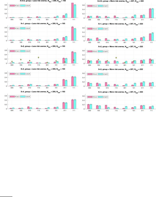
where for simplicity of notation, we write the column vector as a row vector with the transpose operation . The probability for the participant to take the second-stage gamble is obtained by adding the two components ‘Gamble in the second-stage and Won-first- stage belief’ and ‘Gamble in the second-stage and Lost-first-stage belief’

The belief-action state changes by a process based on the available information and is formally controlled by the transition rate matrix K. The specific composition of this matrix causes the transfer of probability between the different belief state components. A main source of transfer in the belief state is the gamble outcome information. Given the belief for ‘Win’ a re-distribution of ‘Gamble’ or ‘Stop’ components will result, and an analogous redistribution will occur given a belief for ‘Lose’. Within the subspace of Win this re-distribution requires a transition rate sub matrix KW , and within the subspace for Lose a transition rate sub matrix KL

14