J.B. Broekaert, et al. |
Cognitive Psychology 117 (2020) 101262 |
parameter {s}, however this parameter is now monitoring a hyperbolic tangent version of the logistic function, Eqs. (41). A similar ‘coupled-switching’ dynamics, controlled by a mixing parameter , is implemented for the attention switching from Win to Lose correlated to switching between Gamble or Stop decision. The mixing Hamiltonian, Eq. (42), and the Markov intensity rate mixing, Eq. (24), are structured differently due to Hermeticity instead of probability conservation requirements. In the gamble block with Win and Lose outcome conditions the context effect is implemented by the weight parameters { , µ} for first period and second period respectively.
In the quantum-like model the carry-over effect from first to second period is implemented differently in the belief-action state for the Unknown condition; instead of weighting two components the parameter { } now causes an interference between the two components by implementing a relative complex phase.
The quantum model, just like the Markov model, relies on 9 parameters to cover the process dynamics and the initial belief-action states in both flow orders, both periods and all payoffs amounting to theoretical values for 30 data points. The Supplementary Materials section, (SM 2) provides more details on the temporal evolution in this model.
4.4. Logistic model
In order to compare the performance of the Markov and quantum-like process models, we devised a third model which aims to heuristically reproduce the observed gamble probabilities. Similarly to the Markov and quantum-like models, this baseline model is also made context and order sensitive but does not comprise a dynamic process for the belief-action state. Instead the baseline model implements for each gamble condition ad hoc weightings of the two utilities for Win outcome and Lose outcome, Eqs. (16). The gamble probability is then simply obtained from a logistic function of the heuristic utility
p (gamble|X, Cond) = |
1 |
|
(50) |
1 + e s·U (X,Cond) |
, |
where the parameter s functions as a sensitivity parameter. In the first period, the utility of taking the second-stage gamble in the Win and in the Lose condition will be set according to
|
|
|
|
|
|
UKU (W ) = KUK uW + (1 |
KUK )uL, |
UKU (L) = (1 |
KUK )uW + KUK uL, |
(51) |
where KUK is a weight parameter, 0 |
KUK |
1, expressing the participant’s inclination towards Win and Lose beliefs. Hence also in |
the Logistic model we allow for partial adherence to the information in the outcome condition, but now this occurs on the level of utility instead of belief probability amplitude. It can be argued that each presented gamble is embedded between Win-outcome and Lose-outcome games, and this engenders residual utility-based support.
In the first period the utility of the Unknown outcome of a first-stage gamble is
UUK (U) = UKU UUK (W ) + (1 UKU )UUK (L) |
(52) |
which expresses the resulting utility is a weighting of Win and Lose conditioned utility assessments, by the parameter  UKU .
UKU .
In the second period the context effect is now modified by the carry-over effect, which changes the weighting in the utility of the Win and Lose outcome gambles
UUK (W ) = UKK uW + (1 UKK )uL, UUK (L) = (1 UKK )uW + UKK uL |
(53) |
in which the weight parameter now is  UKK .
UKK .
In the Unknown first-stage outcome gamble the utility weighting,  KUU , is now changed because of the carry-over effect
UKU (U) = |
KUU UKU (W ) + (1 KUU )UKU (L) |
(54) |
with 0 KUU |
1. |
|
Parametrization. In contrast to the Markov and quantum-like models, the Logistic model does not rely on belief-action states but
rather on heuristically adapted utility functions. For each condition of Known or Unknown outcome, gamble payoff and period a dedicated utility weighting drives a logistic function to render the probabilities for the second-stage gamble. The logistic model
requires the same four dynamical parameters for the driving utility difference as in the two dynamical models, namely { |
0W , 1W } and |
{ 0L, 1L}. The effect of the utility difference on the decision is controlled by a sensitivity parameter {s} on a logistic function, Eq. (50). |
In the |
logistic model the carry-over effect and the context effect are covered by four ad hoc weighting |
parameters, |
{ KUK , |
KUU , UKK , UKU}. |
|
Like the Markov and the quantum-like model, the logistic model uses 9 parameters to produce the gamble probability for both flow orders, both periods and all payoffs amounting to theoretical values for 30 data points.
5. Theoretical model performance
The three models have been parametrized for maximum likelihood statistical estimation on the data set. With three initial gamble outcome conditions and the five variable payoff amounts the survey produces fifteen observed proportions for each block ordering. For each model the objective function G for the parameter optimalisation is
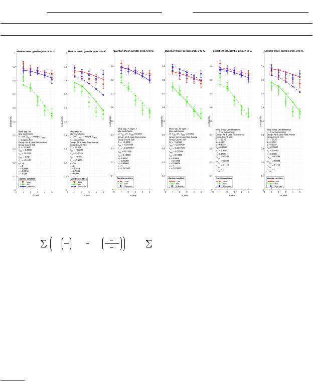
 [1, 5] appears on the x-axis. Error bars represent the standard error of the mean.
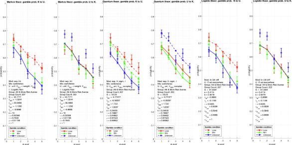
 [1, 5] appears on the x-axis. Error bars represent the standard error of the mean.


 (
( (0), with