Материал: искусственный интеллект

different. On the one hand, the probabilities of Markov processes represent epistemic uncertainty, which is an observer's (e.g., a modeler's) lack of knowledge about the underlying true state existing at each moment in time due to a lack of information about the decision maker's beliefs. On the other hand, the amplitudes of quantum processes represent ontic uncertainty, which is the intrinsic uncertainty about the constructive result that a measurement generates at each moment in time (Atmanspacher, 2002). Ontic uncertainty cannot be reduced by greater knowledge about the decision maker's state.

These are two strikingly different views about the nature of change in belief during evidence accumulation. Markov processes, which include the popular random walk/diffusion models (Diederich & Busemeyer, 2003; Ratcliff et al., 2016), are more established, and have a longer history with many successful applications. These include both the simple random walk models, where a decision maker has a discrete set of states (e.g., 11 confidence levels, 0/10/20/…/100) that they move through over time, shown in Figure 2, and the more common diffusion models where the “states” are a continuously-valued level of evidence (such as 0–100, including all numbers in between). Since the discrete-state random walks approach a diffusion process as the number of states gets very large, we group these two approaches together under the umbrella of Markov process, which have been used to model choices and response times (Emerson, 1970; Luce, 1986; Stone, 1960) as well as probability judgments (Edwards, Lindman, & Savage, 1963; Kvam & Pleskac, 2016; Moran, Teodorescu, & Usher, 2015; Ratcliff & Starns, 2009; Wald & Wolfowitz, 1948; Wald & Wolfowitz, 1949; Yu, Pleskac, & Zeigenfuse, 2015) in domains such as memory (Ratcliff, 1978), categorization (Nosofsky & Palmeri, 1997), and inference (Pleskac & Busemeyer, 2010).

Although quantum processes have a long and successful history in physics, they have only recently been considered for application to human decision making (Busemeyer & Bruza, 2012; Khrennikov, 2010). However, a series of studies have aimed at testing and comparing these two competing views of evidence accumulation. The purpose of this article is to (a) provide an introduction to these two contrasting views, (b) review the research that directly tests and compares these types of theories, and (c) draw conclusions about conditions that determine when each view is more valid, or whether a mixture of the two processes might be needed for a more complete theory.

3 | BASIC PRINCIPLES OF MARKOV AND QUANTUM DYNAMICS

Although the introduction focused on evidence accumulation that occurs during inferential choice problems, Markov and quantum models are based on general principles that can be applied to both evidence and preference accumulation problems. Table 1 provides a side by side comparison of the five general principles upon which the two theories are based. Both theories begin with a set of possible basic states that the system can pass through over time, describing the relative degrees of support for one option or the other. In the case of evidence accumulation, these states are distinct levels of belief. Figure 2 uses 11 levels, but actual applications typically use a much larger number so as to approximate a continuum. In the case of preference accumulation, these states are distinct levels of preference.

State representation principle: For the Markov model, there is a probability distribution across states at each point in time. The probability assigned to each basic state conceptually represents the likelihood that an outside observer might attribute to the decision maker being located at that state. This probability distribution always sums to one. For the quantum model, there is an amplitude distribution across states at each point in time. The amplitude assigned to a basic state can be a real or complex number, and the probability of reporting that state is the squared magnitude of the amplitude.1 The sum of squared amplitudes always sums to one (i.e., the amplitude distribution has unit length). The nonlinear map from amplitudes to probabilities is an important way the two theories differ, and as we will see in the next section on an interference effect, it leads to testable competing predictions.

State evolution principle: For the Markov model, the probability distribution over states evolves for period of time t > 0 according to a linear transition operator. This operator describes the probability of transiting from one basic state to another over some period of time t, representing how incoming information changes the probability distribution over states across time. For the quantum model, the amplitude distribution evolves for a period of time t > 0 according to a linear unitary operator. This operator describes the amplitude for transiting from one basic state to another over some period of time t. Once again, the probability of making this transition is obtained from the squared magnitude. In other applications, the unitary operator can also specify how the state changes according to some fixed amount of new information, such as a single vignette (Trueblood & Busemeyer, 2011) or cue in the choice environment (Busemeyer, Pothos, Franco, & Trueblood, 2011). The unitary operator is required to maintain a unit length amplitude distribution over states across time, thus constraining the sum of squared amplitudes representing the probability of observing different measurement outcome to be equal to one.

Rate of change principle: For the Markov model, the rate of change in the probability distribution is determined by a linear differential equation called the Kolmogorov equation. The integration of these momentary changes are required to form a transition operator. For the quantum model, the rate of change in the amplitude distribution is determined by the Schrödinger equation. The integration of these momentary changes are required to form a unitary operator. These two linear differential equations are not shown here, but they are strikingly similar, except for the complex number i that appears in the Schrödinger equation (which is the reason for using complex amplitudes).

For the Markov model, the linear differential equation is defined by an intensity operator that contains two key parameters: a “drift rate” parameter that determines the direction of change and a “diffusion” parameter that determines the dispersion of the probability distributions. The intensity operator of the Markov model has to satisfy certain properties to guarantee that the linear differential equation produces a transition operator. For the quantum model, the linear differential equation is defined by a Hamiltonian operator that also contains two key parameters: a parameter that determines the “potential function” which controls the direction of change and a “diffusion” parameter that determines the dispersion of the amplitude distribution. The Hamiltonian operator of the quantum model has to satisfy different properties than the intensity operator to guarantee that the linear differential equation produces a unitary operator, but it serves a similar function by evolving the corresponding state according to incoming information. These operators are the key ingredients of any stochastic processing theory and they contain the most important parameters for building a model.

Response selection: For the Markov model, the probability of reporting a response at some point in time equals the sum of the probabilities over the states that map into that response. After observing a response, a new probability distribution, conditioned on the observed response, is formed for future evolution. This probability distribution represents the updated information of an outside observer, where the measurement has reduced their uncertainty about the decision-maker's state. For the quantum model, the probability of reporting a response at some point in time equals the sum of the squared amplitudes over the states that map into that response. After observing a response, a new amplitude distribution, conditioned on the observed response, is formed for future evolution. In quantum models, this conditioning on the observed response is sometimes called the “collapse” of the wave function, which represents a reduction in the ontic uncertainty about the decision maker's evidence level, informing both the decision maker and an outside observer about the decision maker's cognitive state.

Despite the apparent similarities between the quantum and Markov processes outlined in the table, the two processes produce quite distinct behavior. For example, consider two processes shown in Figure 3 again. The Markov process in this figure is analogous to a pile of sand with wind blowing the sand to the right, where the sand eventually piles up in an equilibrium distribution. The quantum process in this figure is more closely analogous to a wave of water with the wind blowing the wave to the right. Once the wave hits the right wall, it bounces back until the wind blows it forward again. The result is that the quantum model does not reach an equilibrium, and instead it oscillates back and forth to the right across time. This interesting behavior is examined later in this article when we discuss preferential evolution. The following sections review previous applications of these models to evidence accumulation problems like choice, confidence, and response time, followed by applications to preference evolution.

4 | INTERFERENCE EFFECTS

The state representation and the response selection process in the Markov process relies on a property that we call the read-out assumption. In Markov models, a judgment or a decision is made by mapping an existing state of evidence onto a response. For instance, a choice is made when evidence reaches a predetermined level of evidence, triggering the appropriate response. Other responses are modeled similarly as a read-out from an existing level of evidence: confidence, for instance, is typically modeled by mapping predetermined levels of evidence to confidence ratings (Moran et al., 2015; Pleskac & Busemeyer, 2010; Ratcliff & Starns, 2009), as are preference ratings (Bhatia & Pleskac, 2019) and judgments like willingness to pay, willingness to accept, and certainty equivalent prices (Johnson & Busemeyer, 2005; Kvam & Busemeyer, 2019).

This read-out assumption bears a striking resemblance to the assumption in economic models that preferences and beliefs are revealed by the choices people make (McFadden, Machina, & Baron, 1999; Samuelson, 1938). Yet decades of research from judgment and decision making and behavioral economics suggests that preferences are not revealed by the choices people make, but rather constructed by the process of generating a response like a choice (Ariely & Norton, 2008; Lichtenstein & Slovic, 2006; Payne, Bettman, & Johnson, 1992; Slovic, 1995). This construction of preference is typically understood as the result of people selecting a specific procedure from a larger repertoire of possible strategies to formulate a response (Gigerenzer et al., 1999; Hertwig et al., 2019; Payne, Bettman, & Johnson, 1993; Tversky, Sattath, & Slovic, 1988), or the dynamic nature of information accumulation that adjusts preferences over time (Busemeyer & Townsend, 1993; Johnson & Busemeyer, 2005). But quantum models, which model a judgment or decision as a measurement process that creates or constructs a definite state from an indefinite (superposition) state, offer a potentially more apt account of this hypothesis that preferences and beliefs are constructed.

5 | INTERFERENCE EFFECTS OF CHOICE ON CONFIDENCE

What are the behavioral implications of this process of constructing a definite state from an indefinite state? If information processing stops after the choice or judgment, then behaviorally this process is hard to dissociate from the classical read-out assumption of Markov models. However, if processing continues after a choice is made, then the two theories can make very different predictions about subsequent judgments. For instance, consider the situation when people are asked to make a choice and then rate their confidence in their choice—such paradigms are common in studies designed to study metacognition and confidence (Lichtenstein, Fischhoff, & Phillips, 1982; Yeung & Summerfield, 2012). If we model evidence accumulation during this situation as a Markov process, then a choice is a read-out of the location of the evidence, and the subsequent confidence judgment is just another read-out. However, we also know that in general evidence accumulation does not stop after the choice and that people continue to collect evidence after their choice (Baranski & Petrusic, 1998; Moran et al., 2015; Pleskac & Busemeyer, 2010; Yu et al., 2015). Consequently, a confidence judgment is made based on the evidence accumulated to make a choice as well as the evidence from postdecisional processing. Because classical models of evidence accumulation do not change the state of the evidence when it is measured, making a choice does not have an impact on the confidence people report. Thus, if a choice is made, but we ignore the choice, then the confidence should be the same as if they made no choice at all. In comparison, in a quantum process, a choice does changes the state of the evidence when a choice is made, and so even if we ignore the choice, the simple act of measurement does impact confidence judgments following subsequent evidence accumulation.

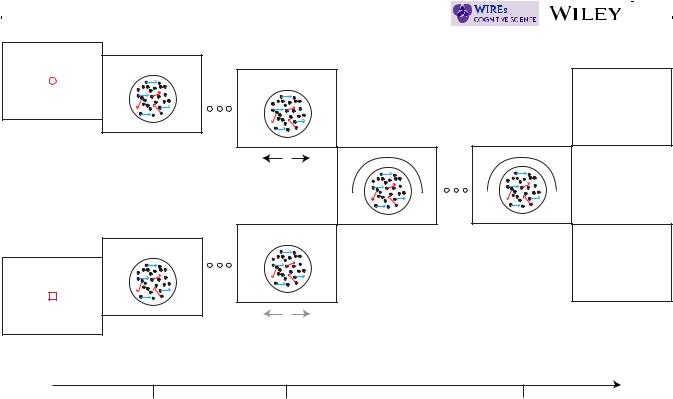
These are parameter-free competing predictions that hold for a large range of evidence accumulation processes, including ones where there is decay and trial-by-trial variability (for a mathematical proof, see Kvam et al., 2015). In general, they arise from the first-principles of each of the theories. To get an intuitive feel for the predictions, consider the experiment shown in Figure 4 that Kvam et al. (2015) asked participants to complete. In the experiment, participants viewed a random dot motion stimulus where a percentage of the dots moved coherently in one direction (left or right), and the rest moved randomly. In half of the blocks of trials participants were prompted at time point t1 (0.5 s) to decide whether the coherently moving dots were moving left or right and entered their choice via a mouse. In the the other half of the blocks—the no-choice condition—participants were prompted at t1 to click a predetermined mouse button. In all the trials, at a second time point t2, participants were prompted to rate their confidence that the coherently moving dots were moving right ranging from 0% (certain left) to 100% (certain right).

The prediction of no interference from the Markov model arises because it models evidence accumulation as the evolution of the probability distribution over evidence levels across time. In the choice condition, according to the