Материал: Russian Journal of Building Construction and Architecture
Issue № 3 (43), 2019 |
ISSN 2542-0526 |
900
P, kPа
800
700
R² = 0.8545
600
500 
400
300
200
100
0 |
|
|
|
|
|
|
|
|
|
|
|
|
|
|
|
|
|
|
|
|
|
|
|
|
|
|
|
|
|
N, Hz |
||
|
|
|
|
|
|
|
|
|
||
0 |
0,5 |
11 |
2 1,5 |
3 |
2 |
4 |
2,5 |
3 |
||
|
||||||||||
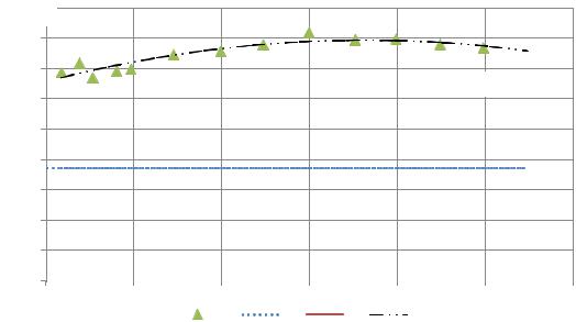
Fig. 6. Pressure changes at the characteristic points of a closed hydraulic contour in relation to the atmospheric pressure when available head pressure is maintained at 130 kPа when the frequencies of valve switching of the shock node change: 1 is the maximum pressure growth at the moment of the hydraulic shock (experimental data); 2 is the averaged pressure at the inlet of the pump;
3 is the averaged pressure at the outlet of the pump; 4 is Excel approximation for the dataset 1
Fig. 6 suggests that the pressure growth at the moment of the hydraulic shock has a distinct maximum at the frequency of around 1.5 Hz. This is due to the fact that at a smaller frequency of valve switching, which characterizes their smoothness an incomplete hydraulic shock. At a higher frequency of valve switching the consumption of the operating environment through the shock node is not able to reach its maximum corresponding with the available head pressure of 130 kPа and resistance of the hydraulic system.
4. Mathematical modeling of the shock node. Reliable and efficient reaction of a shock node during generation of periodic hydraulic shocks in a certain setup is characterized by the closing time of the valve t, seс which should be less than some design value tp, seс when a hydraulic shock wave reaches the distance equaling two alimentary pipe lengths. The valve should close before a reflected hydraulic shock wave reaches it when it is open, i. e. the following equation should hold
t tр |
2L |
, |
(1) |
|
a |
|
|
where t is the current closing time of the valve, seс; tp is the design closing time of the valve, seс; L is the length of an alimentary pipe, m; a is the distribution rate of the hydraulic shock wave, m/seс.
25
Russian Journal of Building Construction and Architecture
The current closing time t, seс of the valve of the hydraulic shock should be given by changes in the rate v, m/seс using the ratio
t |
|
, |
(2) |
|
|
||
|
v |
|
|
whereδ isa gap betweenthe valve seat and the valve itself, m; |
v is change in the rate, m/seс. |
||
Change in the rate v, m/seс, can be predicted using the amplitude and frequency characteristics obtained using the force and rate growth. These characteristics are easy to design energy chains are used.
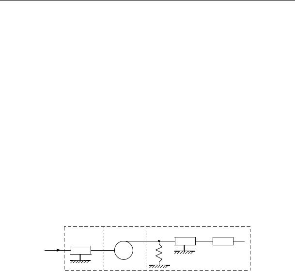
The energy chain of the shock node when the valve closes has 3 links (Fig. 7): the first one is hydraulic which accounts for the hydraulic resistance of the valve using the active resistance r1, (kPа·seс2)/l2; the second one is transformative, it transforms the pressure Р1, kPа, and the volumetric consumption V, l/sec, into the force f, H, and the linear rate v, m/sec, respectively; the third link is mechanical, it accounts for the properties of the spring-loaded valve with the deformation l, m/Н, mechanical friction for active resistance friction r2, (Н·seс)/m, and inertia properties with the mass т, kg, of moving parts of the valve.
1 2 3
|
r1 P1 |
f |
r2 |
f |
m f |
2 |
P |
v |
|
1 |
|
||
v1 |
v1 |
v1 |
||||
V |
V |
|
l |
|
|
|
Fig. 7. Energy chain of the shock node when the valve closes: P is the pressure of the operating environment at the inlet of the shock valve, kPa; V is the volumetric consumption of the operating environment through the shock node, l/sec; r1 is the hydraulic (active) resistance of the valve, (kPа·seс2)/l2; Р1 is the pressure of the operating environment at the outlet of the valve considering the hydraulic (active) resistance of the valve, kPа; f is the force on the valve from the inlet of the operating environment, H; v is the linear closing rate of the valve, m/seс; l is the deformation of the spring-loaded valve, m/Н; v1 is the linear closing rate of the valve considering a
drop in the rate of its deformation, m/seс; r2 is the mechanical (active) resistance of the valve, (Н·seс)/m; f1 is the force of the valve from the inlet of the operating environment, H; m is the mass of the valve and other moving parts of the shock node, kg; f2 is the force on the valve from the inlet of the operating environment, H;
S is the section area of the valve, mm2
The equations of the links of this chain are as follows:
|
1 |
|
2 |
P rV2 |
P; |
P f / S; |
|
|
1 |
1 |
1 |
V V. |
|
V vS. |
|
3
f rv m v |
1 |
f |
2 |
; |
(3) |
|||
|
2 |
1 |
2 |
|
|
|||
|
v lf v . |
|
|
|
|
|
||
|
|
|
|
|
|
|||
|
|
|
1 |
|
|
|
|
|
26
Issue № 3 (43), 2019 |
ISSN 2542-0526 |
Let us present the outlet parameters of the chain as the sum of the constant component and deviation:
f2 f20 |
|
|
|
|
v1 v20 v1. |
(4) |
|||||||||
f2, |
|
|
|||||||||||||
Then the equation for Р1 is as follows: |
|
|
|
|
|
|
|
|
|
|
|
||||
|
1 |
|
|
|
1 |
|
|
|
|
1 |
|
|
|
, |
(5) |
|
|
|
|
|
|
|
|
|
|
||||||
P |
|
r v |
|
m v |
|
|
|
f |
|
|
|
||||
1 |
S 2 1 |
|
2 1 |
|
|
2 |
|
|
|||||||
and the equation for V is transformed into |
|
|
|
|
|
|
|
|
|
||||||
V Slf |
Sv |
Sv . |
|
|
|
(6) |
|||||||||
|
|
|
|
|
|
|
20 |
|
|
1 |
|
|
|
|
|
Using the substitute
f r2v1 m2v1 f2,
we get
V Slr2v1 Slm2v1 Slf2 Sv20 Sv1.
And
V 2 S 2v |
2 |
|
2S |
2v lr v |
|
2S 2v lmv |
|
2S |
2v lf |
2S2v v . |
|
||||||||||||||||||||||||||||||||||||||||
|
|
|
20 |
|
|
|
|
20 |
2 |
|
1 |
|
|
|
|
|
20 |
|
1 |
|
|
|
|
20 |
2 |
|
|
|
|
|
|
|
|
20 |
1 |
|
|
||||||||||||||
Into the equation P |
|
|
|
|
|
|
|
|
|
|
|
|
|
|
|
|
|
|
|
|
|
|
|
|
|
|
|
|
|
|
|
|
|
|
|
|
|
|
|
|
|
|
|
|
|
|
|
|
|
||
P r S |
2v2 2S |
2r v lr v |
2S2v rlmv |
2S 2v v lf |
|
|
2S |
2v r v |
1 r v |
||||||||||||||||||||||||||||||||||||||||||
1 |
|
20 |
|
|
|
1 20 2 1 |
|
|
|
|
|
|
|
|
20 1 |
|
1 |
|
|
|
|
|
20 1 2 |
|
|
|
|
|
|
|
|
20 1 1 |
|
2 1 |
|||||||||||||||||
|
1 |
|
|
|
1 |
|
|
|
|
|
1 |
|
|
|
|
|
|
|
|
1 |
|
|
2S |
2 |
|
|
|
|
|
|
|
2S |
2 |
|
|
|
|
|
|
|
|
||||||||||
|
|
|
|
|
|
|
|
|
|
|
|
|
|
|
|
|
|
|
|
|
|
|
|
|
|
|
|
|
|
|
|||||||||||||||||||||
|
|
r v |
|
|
mv |
|
|
|
S |
|
f |
|
|
|
|
S |
f |
|
|
|
v rlmv |
|
|
|
r v lr v |
|
|||||||||||||||||||||||||
|
2 20 |
|
|
|
1 |
|
|
|
|
|
2 |
|
|
|
|
|
20 |
|
|
|
|
|
|
|
20 1 |
|
|
1 |
|
|
|
|
|
|
|
|
1 20 2 |
|
|
||||||||||||
|
|
(2S |
2 |
|
|
|
|
|
1 |
|
|
|
)v |
|
|
|
|
1 |
|
|
|
2S |
2 |
|
|
|
|
|
|
|
1 |
|
|
|
|
|
|
1 |
|
|
|
|
|
||||||||
|
|
|
|
|
|
|
|
|
|
|
|
|
|
|
|
|
|
|
|
|
|
|
|
|
|
|
|
|
|
|
|
|
|||||||||||||||||||
|
|
|
v r |
|
|
|
|
r |
|
|
|
|
r v |
|
|
|
v rlf |
|
|
|
|
f |
|
|
|
|
|
|
f |
|
|
|
|||||||||||||||||||
|
|
|
|
S |
|
|
|
S |
|
|
|
|
S |
|
|
|
S |
|
|
|
|
||||||||||||||||||||||||||||||
|
|
|
|
|
20 1 |
|
|
|
2 1 |
|
|
|
|
2 20 |
|
|
|
|
|
|
20 1 2 |
|
|
|
|
|
2 |
|
|
|
20 |
|
|
||||||||||||||||||
the following coefficients are introduced: |
|
|
|
|
|
|
|
|
|
|
|
|
|
|
|
|
|
|
|
|
|
|
|
|
|
|
|
|
|||||||||||||||||||||||
a 2S2v rlm; a 2S2rv lr ; |
a 2S 2v r |
|
1 |
r ; a |
|
|
|
|
1 |
r v ; |
|||||||||||||||||||||||||||||||||||||||||
|
|
|
|
|
S |
||||||||||||||||||||||||||||||||||||||||||||||
1 |
|
20 1 |
|
|
|
|
2 |
|
|
|
|
|
|
1 20 2 |
|
3 |
|
|
|
|
|
|
20 1 |
|
|
|
S 2 |
|
|
|
|
4 |
|
|
|
|
2 20 |
||||||||||||||
|
|
|
|
|
|
|
|
b 2S2v rl; |
b |
1 |
; b |
1 |
, |
|
|
|
|
|
|
|
|
|
|
|
|
|
|
|
|
|
|||||||||||||||||||||
|
|
|
|
|
|
|
|
1 |
|
|
|
|
|
|
|
|
|
|
20 1 |
|
2 |
|
|
S |
|
|
|
|
3 |
S |
|
|
|
|
|
|
|
|
|
|
|
|
|
|
|
|
|
||||
|
|
|
|
|
|
|
|
|
|
|
|
|
|
|
|
|
|
|
|
|
|
|
|
|
|
|
|
|
|
|
|
|
|
|
|
|
|
|
|
|
|
|
|
|
|
|
|
||||
and by grouping them in the equation (10), we get
P a1v1 a2v1 a3v1 a4 b1 f2 b2 f2 b3.
The equation for the images is as follows:
(b1 f2 b2 f2 b3)F2(s) (a1v1 a2v1 a3v1 a4)V1(s).
The complex resistance of the chain is given by the expression
Z (s) |
v1(s) |
|
b1s b2 |
|
. |
|
F (s) |
|
|
||||
|
|
a s2 |
a s a |
|
||
|
2 |
|
1 |
2 |
3 |
|
(7)
(8)
(9)
(10)
(11)
(12)
(13)
(14)
(15)
27
Russian Journal of Building Construction and Architecture
The frequency function of the chain:
Z ( j ) a1 b21 j a2 jb2 a3 . The valid part of the frequency function:
Re(j ) a2b1 22 b2a1 2 2 2b2a23 .
( a1 a3) a2
The imaginary part of the frequency characteristics:
Im(j ) b1a1 32 b1a32 b22a22 j.
( a1 a3) a2
The amplitude and frequency characteristics of the chain:
(16)
(17)
(18)
A( j ) Re( j )2 Im( j )2 . |
(19) |
The basic parameters for the scheme of the experimental setup are as follows: r1 = 50 (kPа seс2)/l2; r2 = 1 (Н seс)/m; l = 0.075 m/Н; т = 0.15 kg; S = 490.625 mm2 (at the valve diameter d = 25 mm); V20 = 0.2 l/seс.
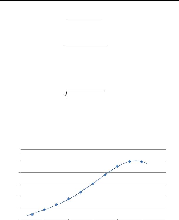
Based on the expressions (17)––(19) the graph of the amplitude and frequency characteristics will be as presented in Fig. 8.
A1,2(jΩ)
1
R² = 0.9997
0,8
0,6
0,4
0,2
0
0 |
2 |
4 |
6 |
8 |
10 |
Ω, rad/sec12 |
Fig. 8. Amplitude and frequency characteristics of the energy chain when the valve closes with the basic parameters of the energy chain
Fig. 8 suggests that the amplitude and frequency characteristics A(jΩ) reaches its maximum at the angular rate Ω ≈ 9.4 rad/seс, which corresponds with the cam frequency f = 1.49 Hz and rate change v = 1 m/seс. Considering the actual gap between the valve and its seat δ = 5 mm,
28
Issue № 3 (43), 2019 |
ISSN 2542-0526 |
based on the formula (2) the current closing time of the valve at the moment is t 0.0051 0.005sek.
The design time for reaching the effective operation of the hydroshock node at the alimentary pipe length L = 1.3 m and the distribution rate of the hydraulic shock in a PP-R pipe а = 398 m/seс given by the formula by N. Ye. Zhukovskiy [6, p. 105] based on the formula
(1) we get
tр 2 1.3 0.0065 sek. 398
Since at the angular speed Ω ≈ 9,4 rad/seс the time is t > tp, the shock node will operate effectively according to the mathematical modeling condition (1).
The sufficiency of the mathematical modeling is proved by the results of experimental studies presented in Fig. 6 where the maximum pressure increases at the moment of the hydraulic shock was also observed at the valve switching frequency of around f = 1.5 Hz. Considering that, Fig. 9––12 present the results of mathematical modeling of the shock node when the valve closes with a variation in the most significant parameters of the energy chain according to the Table.
|
|
|
|
|
|
|
Таble |
|
|
|
Modeling parameters |
|
|
|
|
|
|
|
|
|
|
|
|
№ |
r1, |
r2, |
l, m/Н |
|
т, kg |
V20, l/sec |
Graphs |
(kPа seс2)/l2 |
(Н seс)/m |
|
|||||
|
|
|
|
|
|
||
1 |
50 |
1 |
0.075 |
|
0.1 |
0.2 |
|
|
|
|
|
|
|
|
Fig. 9 |
2 |
50 |
1 |
0.075 |
|
0.15 |
0.2 |
|
|
|
|
|
|
|
|
|
3 |
50 |
1 |
0.075 |
|
1 |
0.2 |
|
|
|
|
|
|
|
|
|
4 |
50 |
1 |
0.05 |
|
0.15 |
0.2 |
|
|
|
|
|
|
|
|
Fig. 10 |
5 |
50 |
1 |
0.075 |
|
0.15 |
0.2 |
|
|
|
|
|
|
|
|
|
6 |
50 |
1 |
1 |
|
0.15 |
0.2 |
|
|
|
|
|
|
|
|
|
7 |
50 |
1 |
0.075 |
|
0.15 |
0.1 |
|
|
|
|
|
|
|
|
Fig. 11 |
8 |
50 |
1 |
0.075 |
|
0.15 |
0.2 |
|
|
|
|
|
|
|
|
|
9 |
50 |
1 |
0.075 |
|
0.15 |
100 |
|
|
|
|
|
|
|
|
|
10 |
50 |
0.5 |
0.075 |
|
0.15 |
0.2 |
|
|
|
|
|
|
|
|
Fig. 12 |
11 |
50 |
1 |
0.075 |
|
0.15 |
0.2 |
|
|
|
|
|
|
|
|
|
12 |
50 |
1.5 |
0.075 |
|
0.15 |
0.2 |
|
|
|
|
|
|
|
|
|
Fig. 9 suggests that as the mass of the moving parts of the shock node increases, the maximum possible rate change at the moment of the hydraulic shock v, m/seс, decreases and so
29