Материал: Russian Journal of Building Construction and Architecture

Issue № 3 (43), 2019 |
ISSN 2542-0526 |
3. Natural experiments of statistical laws of the distribution of the elasticity modulus s and damping coefficients of flexible road pavements. Possible restoration of the parameters of the dynamic strain-stress of road pavements using the results of instrumental evaluation and mechanic and mathematical modeling allows their actual condition to be evaluated in accordance to the design project. It should be noted, however, that in order to do this, it is necessary that the statistical laws of the distribution of the major structural parameters of flexible road pavements and laws of their degradation throughout the life cycle.
In order to solve this problem, from 2014 to 2018 studies were conducted in the operating areas of the highways so that the statistical laws of the distribution of the major structural parameters (elasticity modulus s and damping coefficients) of flexible road pavements and their change during operation were identified. For this purpose, all the investigated areas of the highways were divided into three groups with the life cycle of 0––5 years, 5––10 years, over 10 years. The total length of the investigated areas was 260 km where over 3000 deflection bowls and amplitude-time characteristics of displacements were recorded. According to the analysis of the results, it was found that the distribution of the elasticity modulus and damping coefficients of flexible road pavements obeys the logarithmically normal law:
f t |
|
1 |
|
e |
lnt m 2 |
|
|
|
2 2 , |
(4) |
|||
t |
|
2 |
||||
|
|
|
|
|
where m and σ are the parameters of the logarithmically normal distribution (scale parameters and distribution forms).
Based on the measurements, the averaged parameters of the logarithmically normal distribution for road pavements with the life cycle of 0––5 years, 5––10 years, 10––15 years (Table 1––2).
Таble 1
Average values of the parameters of the logarithmically normal distribution of the elasticity modulus s of construction layers of road pavements for different types of areas
|
|
|
Groups of the investigated area |
|
||
Statistical parameter |
|
|
|
|
|
|
Group I (with the life |
|
Group II (with the life |
|
Group III (with the life |
||
|
|
cycleof less than 5 years) |
|
cycle of 5––10 years) |
|
cycle of over 10 years) |
|
|
|
|
|
|
|
Asphalt |
m |
7.96 |
|
7.41 |
|
7.34 |
concrete |
|
|
|
|
|
|
σ |
0.20 |
|
0.24 |
|
0.36 |
|
|
|
|
|
|
|
|
Foundation |
m |
5.65 |
|
5.24 |
|
5.10 |
|
|
|
|
|
|
|
σ |
0.20 |
|
0.25 |
|
0.37 |
|
|
|
|
||||
|
|
|
|
|
|
|
Subgrade soil |
m |
4.30 |
|
4.10 |
|
4.02 |
|
|
|
|
|
|
|
σ |
0.15 |
|
0.20 |
|
0.23 |
|
|
|
|
||||
|
|
|
|
|
|
|
85

Russian Journal of Building Construction and Architecture
Таble 2
Average parameters of the logarithmically normal distribution of the damping coefficients of road pavement layers for different types of areas
Statistical |
|
Groups of the investigated area |
|
||
|
|
|
|
|
|
parameter |
|
Group I (with the life cycle |
Group II (with the life |
|
Group III (with the life |
|
of less than 5 years) |
cycle of 5––10 years) |
|
cycle of over 10 years) |
|
|
|
|
|||
|
|
|
|
|
|
Asphalt |
m |
–2.79 |
–2.18 |
|
–1.63 |
concrete |
|
|
|
|
|
σ |
0.29 |
0.33 |
|
0.40 |
|
|
|
|
|
|
|
Foundation |
m |
–3.54 |
–3.07 |
|
–2.72 |
|
|
|
|
|
|
σ |
0.31 |
0.31 |
|
0.36 |
|
|
|
||||
|
|
|
|
|
|
Subgrade soil |
m |
–3.36 |
–3.83 |
|
–3.89 |
|
|
|
|
|
|
σ |
0.25 |
0.22 |
|
0.22 |
|
|
|
||||
|
|
|
|
|
|
The obtained averaged parameters of the logarithmically normal distribution are the foundation for modeling changes in the dynamic contour of hysteresis loops on the road pavement surface at different stages of its operation and are accounted for in determining the calculated and residual resources of road pavements.
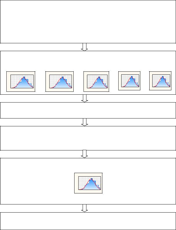
4. Тheoretical foundations of the implementation of the system of technical monitoring of road pavements. A set of theoretical and natural experiments allowed the main approaches to be formulated that are set forth as part of the system of technical monitoring of flexible road pavements including three major sections (Fig. 3––5).
––determining the calculated contour (development) of road pavements throughout its life cycle;
––identifying the residual resource and gamma-percentage resource of road pavements, evaluation of design solutions;
––specifying the thickness of the reinforcement of road pavements for its design life cycle. The suggested approaches rely on calculating the total dissipated energy in the road pavement structure throughout its life cycle based on calculating dynamic hysteresis loops over a loading cycle under the calculated vehicle’s wheel considering the statistical laws of the distribution of the major structural and operational parameters of flexible road pavements (Fig. 3). The use of the modern equipment enabling the major structural and operational parameters of flexible road pavements to be determined allows one to calculate the actual dynamic stress-strain of road pavements at their operation stage followed by calculations of actual dynamic hysteresis loops of the road structure and identifying its actual development before the experiments got underway.
86
Issue № 3 (43), 2019 |
ISSN 2542-0526 |
Input data:
Road structure:
Elasticity modulus s of the layers E1…En
Thickness of the layers h1…hn
Damping coefficients λ1…λn
Longitudinal evenness IRI
Transport load:
Total number of calculated load applications –– 115 kN
Statistical modeling of the input data based on the laws of the degradation of the highways identified in the natural experiments
E1…En
|
|
|
|
|
|
Hist ogram of |
Var3 |
|
|
|
|
|
|
||
|
|
|
Var3 = 100*2. 0000*Normal(x, 15. 2698,4. 9841) |
|
|
|
|
||||||||
|
20 |
|
|
|
|
|
|
|
|
|
|
|
|
|
|
|
18 |
|
|
|
|
|
|
|
|
|
|
|
|
|
|
|
16 |
|
|
|
|
|
|
|
|
|
|
|
|
|
|
of Observations |
14 |
|
|
|
|
|
|
|
|
|
|
|
|
|
|
12 |
|
|
|
|
|
|
|
|
|
|
|
|
|
|
|
10 |
|
|
|
|
|
|
|
|
|
|
|
|
|
|
|
8 |
|
|
|
|
|
|
|
|
|
|
|
|
|
|
|
No |
6 |
|
|
|
|
|
|
|
|
|
|
|
|
|
|
|
4 |
|
|
|
|
|
|
|
|
|
|
|
|
|
|
|
2 |
|
|
|
|
|
|
|
|
|
|
|
|
|
|
|
0 |
|
|
|
|
|
|
|
|
|
|
|
|
|
|
|
0 |
2 |
4 |
6 |
8 |
10 |
12 |
14 |
16 |
18 |
20 |
22 |
24 |
26 |
28 |
|
|
|
|
|
|
|
Var3 |
|
|
|
|
|
|
|
|
h1...hn
|
|
|
|
|
|
Histogram of |
Var3 |
|
|
|
|
|
|
||
|
|
|
Var3 = 100*2. 0000*Normal( x, 15. 2698, 4. 9841) |
|
|
|
|
||||||||
|
20 |
|
|
|
|
|
|
|
|
|
|
|
|
|
|
|
18 |
|
|
|
|
|
|
|
|
|
|
|
|
|
|
|
16 |
|
|
|
|
|
|
|
|
|
|
|
|
|
|
of Observations |
14 |
|
|
|
|
|
|
|
|
|
|
|
|
|
|
12 |
|
|
|
|
|
|
|
|
|
|
|
|
|
|
|
10 |
|
|
|
|
|
|
|
|
|
|
|
|
|
|
|
8 |
|
|
|
|
|
|
|
|
|
|
|
|
|
|
|
No |
6 |
|
|
|
|
|
|
|
|
|
|
|
|
|
|
|
4 |
|
|
|
|
|
|
|
|
|
|
|
|
|
|
|
2 |
|
|
|
|
|
|
|
|
|
|
|
|
|
|
|
0 |
|
|
|
|
|
|
|
|
|
|
|
|
|
|
|
0 |
2 |
4 |
6 |
8 |
10 |
12 |
14 |
16 |
18 |
20 |
22 |
24 |
26 |
28 |
|
|
|
|
|
|
|
Var3 |
|
|
|
|
|
|
|
|
λ1…λn
|
|
|
|
|
|
Histogram of |
Var3 |
|
|
|
|
|
|
||
|
|
|
Var3 = 100*2. 0000*Normal(x, 15.2698, 4. 9841) |
|
|
|
|
||||||||
|
20 |
|
|
|
|
|
|
|
|
|
|
|
|
|
|
|
18 |
|
|
|
|
|
|
|
|
|
|
|
|
|
|
|
16 |
|
|
|
|
|
|
|
|
|
|
|
|
|
|
vatonsi |
14 |
|
|
|
|
|
|
|
|
|
|
|
|
|
|
12 |
|
|
|
|
|
|
|
|
|
|
|
|
|
|
|
of Obser |
10 |
|
|
|
|
|
|
|
|
|
|
|
|
|
|
8 |
|
|
|
|
|
|
|
|
|
|
|
|
|
|
|
No |
6 |
|
|
|
|
|
|
|
|
|
|
|
|
|
|
|
4 |
|
|
|
|
|
|
|
|
|
|
|
|
|
|
|
2 |
|
|
|
|
|
|
|
|
|
|
|
|
|
|
|
0 |
|
|
|
|
|
|
|
|
|
|
|
|
|
|
|
0 |
2 |
4 |
6 |
8 |
10 |
12 |
14 |
16 |
18 |
20 |
22 |
24 |
26 |
28 |
|
|
|
|
|
|
|
Var3 |
|
|
|
|
|
|
|
|
ΣNр
|
|
|
|
|
|
Histogram of |
Var3 |
|
|
|
|
|
|
||
|
|
|
Var3 = 100*2.0000*Normal(x,15.2698, 4.9841) |
|
|
|
|
||||||||
|
20 |
|
|
|
|
|
|
|
|
|
|
|
|
|
|
|
18 |
|
|
|
|
|
|
|
|
|
|
|
|
|
|
|
16 |
|
|
|
|
|
|
|
|
|
|
|
|
|
|
vatonsi |
14 |
|
|
|
|
|
|
|
|
|
|
|
|
|
|
12 |
|
|
|
|
|
|
|
|
|
|
|
|
|
|
|
Obser |
10 |
|
|
|
|
|
|
|
|
|
|
|
|
|
|
of |
8 |
|
|
|
|
|
|
|
|
|
|
|
|
|
|
No |
6 |
|
|
|
|
|
|
|
|
|
|
|
|
|
|
|
4 |
|
|
|
|
|
|
|
|
|
|
|
|
|
|
|
2 |
|
|
|
|
|
|
|
|
|
|
|
|
|
|
|
0 |
|
|
|
|
|
|
|
|
|
|
|
|
|
|
|
0 |
2 |
4 |
6 |
8 |
10 |
12 |
14 |
16 |
18 |
20 |
22 |
24 |
26 |
28 |
|
|
|
|
|
|
|
Var3 |
|
|
|
|
|
|
|
|
IRI
|
|
|
|
|
|
Histogram of |
Var3 |
|
|
|
|
|
|
||
|
|
|
Var3 = 100*2.0000*Normal(x,15.2698, 4.9841) |
|
|
|
|
||||||||
|
20 |
|
|
|
|
|
|
|
|
|
|
|
|
|
|
|
18 |
|
|
|
|
|
|
|
|
|
|
|
|
|
|
|
16 |
|
|
|
|
|
|
|
|
|
|
|
|
|
|
vatonsi |
14 |
|
|
|
|
|
|
|
|
|
|
|
|
|
|
12 |
|
|
|
|
|
|
|
|
|
|
|
|
|
|
|
Obser |
10 |
|
|
|
|
|
|
|
|
|
|
|
|
|
|
of |
8 |
|
|
|
|
|
|
|
|
|
|
|
|
|
|
No |
6 |
|
|
|
|
|
|
|
|
|
|
|
|
|
|
|
4 |
|
|
|
|
|
|
|
|
|
|
|
|
|
|
|
2 |
|
|
|
|
|
|
|
|
|
|
|
|
|
|
|
0 |
|
|
|
|
|
|
|
|
|
|
|
|
|
|
|
0 |
2 |
4 |
6 |
8 |
10 |
12 |
14 |
16 |
18 |
20 |
22 |
24 |
26 |
28 |
|
|
|
|
|
|
|
Var3 |
|
|
|
|
|
|
|
|
Analysis of the dynamic stress-strain of the road structure using the analytical model for the investigated combinations of the input parameters
Calculating the density of the dissipated energy under the calculated vehicle’s wheel for each year of the life cycle of the road structure based on the dynamic hysteresis loops designed
for the investigated combinations of the input parameters in the spatial setting:
Wxx (σxx εxx ), |
Wyy (σyy εyy ), |
Wzz.пр (σzz εzz ) |
Summing the density of the dissipated energy on the road structure surface throughout the life cycle for the investigated combinations of the input parameters
|
|
|
|
|
|
|
Histogram |
of Var3 |
|
|
|
|
|
|
||
|
|
|
|
Var3 = 100*2. 0000*Normal(x, 15. 2698, 4. 9841) |
|
|
|
|
||||||||
|
|
20 |
|
|
|
|
|
|
|
|
|
|
|
|
|
|
|
|
18 |
|
|
|
|
|
|
|
|
|
|
|
|
|
|
|
|
16 |
|
|
|
|
|
|
|
|
|
|
|
|
|
|
|
onsi |
14 |
|
|
|
|
|
|
|
|
|
|
|
|
|
|
|
|
|
|
|
|
|
|
|
|
|
|
|
|
|
|
|
|
of Observat |
12 |
|
|
|
|
|
|
|
|
|
|
|
|
|
|
|
10 |
|
|
|
|
|
|
|
|
|
|
|
|
|
|
|
|
8 |
|
|
|
|
|
|
|
|
|
|
|
|
|
|
|
|
No |
6 |
|
|
|
|
|
|
|
|
|
|
|
|
|
|
|
|
4 |
|
|
|
|
|
|
|
|
|
|
|
|
|
|
|
|
2 |
|
|
|
|
|
|
|
|
|
|
|
|
|
|
|
|
0 |
|
|
|
|
|
|
|
|
|
|
|
|
|
|
|
|
0 |
2 |
4 |
6 |
8 |
10 |
12 |
14 |
16 |
18 |
20 |
22 |
24 |
26 |
28 |
|
|
|
|
|
|
|
|
Var3 |
|
|
|
|
|
|
|
|
W i |
W i |
|
|
|
W i |
|
|
W i |
||||||||
пр |
|
|
xx.пр |
|
|
|
|
yy.пр |
|
|
zz.пр |
|||||
Determining the calculated development as the total density of the dissipated energy in the road pavement throughout the life cycle of the specified level
95 % (Category I), 90 % (Category II), 80 % (Category III)
Fig. 3. Determining the calculated total development of the road pavement at the design stage
The difference between the calculated development of the road pavement determined in accordance with the algorithm in Fig. 3 and actual development identified at the construction stage allows the residual resource of the road structure to be calculated (Fig. 4).
87

Russian Journal of Building Construction and Architecture
Operation stage
Evaluation of the structural parameters of the road structure at the operation stage:
––elasticity modulus of the asphalt concrete layer;
––elasticity modulus
of the foundation layer;
–– elasticity modulus of the subgrade soil
–– damping coefficient
of the asphalt concrete layer;
––damping coefficient of the foundation layer;
––damping coefficient of the subgrade soil;
––damping coefficients of the layers
Evaluation of actual longitudinal evenness of the road pavement surfacing
Analysis of the dynamic stress-strain of the road structure using the analytical model for actual parameters of the road structure specified at the operation stage:
эксплxx ( xx ), |
эксплyy ( yy ), |
эксплzz ( zz ) |
Calculating the density of the dissipated energy under the calculated vehicle’s wheel for each year of the life cycle of the road structure based on the dynamic hysteresis loops in the spatial setting designed for the actual parameters specified at the operation stage:
Wxx.экспл( xx xx ), |
Wyy.экспл ( yy yy ), |
Wzz.экспл( zz zz ) |
Determining the total density of the dissipated energy in the road structure throughout the operation
period: W'экспл (Wxx.экспл Wyy.экспл Wzz.экспл ) N р
Calculation of the residual density of the dissipated energy transferred during vehicle movement:
W'ост Wполн Wэкспл
Calculation of the residual resource, residual life cycle, gamma-percentage residual resource, gamma-percentage residual life cycle
Fig.4. Determiningtheindices of theresidualresourceandresiduallife cycleof roadpavements attheoperationstage
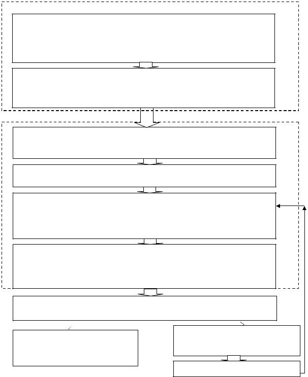
Using the suggested approach the thickness of the reinforcement layer of road pavements can be determined that would allow the density of the energy dissipated on the surface of flexible road pavements to be reduced to the calculated (design) level (Fig. 5).
88
Issue № 3 (43), 2019 |
ISSN 2542-0526 |
Designing stage
Analysis of the dynamic stress-strain of the road structure under the calculated vehicle’s wheel for the design parameters of theroadstructure based on its life cycle:
Wxx.пр ( xx xx ), |
Wyy.пр ( yy yy ), |
Wzz.пр ( zz zz ) |
Determining the density of the dissipated energy under the calculated vehicle’s wheel based on the life cycle of the road structure:
Wпрi Wxxi .пр Wyyi .пр Wzzi .пр
Operation stage
Monitoring the operational condition of the road structure while measuring the structural parameters of the road structure
Identifying the characteristic sections of the road pavements based on the monitoring results
Analysis of the dynamic stress-strain of the road structure under the calculated vehicle’s wheel for the operational parameters of the road structure based on its life cycle:
Wxx.факт( xx xx), |
Wyy.факт( yy yy), |
Wzz.факт( zz zz ) |
Determining the density of the dissipated energy under the calculated vehicle’s wheel based on the life cycle of the road structure:
Wфактi Wxxi .факт Wyyi .факт Wzzi .факт
Comparison of Wпрi and Wфактi
Wпрi Wфактi –– the structure is operational
Wпрi Wфактi –– the structure is not operational
Choosing the thickness of the layer
Fig. 5. Method of the design of the reinforcement measures of road pavements
The approach was tested in one of the operated areas of the highway М-4 Don. The structure of the road pavement in this area is shown in Fig. 6. The total number of the calculated loads for the structure was 12 233 000 calculation loads А11.5 (115 kN) throughout the life cycle.
89