Материал: искусственный интеллект

6Maximum Expected Utility in Quantum-Like Influence Diagrams

The proposed quantum-like influence diagram is built upon the formalisms of quantum-like Bayesian networks. This means that real classical probabilities need to be replaced by complex quantum amplitudes.

We start the derivation with the initial notion of expected utility already presented in the previous section. In a decision scenario, D, given a set of possible decision rules, δA, the goal of the Quantum-Like Influence Diagrams is to compute the decision rule that leads to the Maximum Expected Utility. P rδA (x|a) corresponds to a full joint probability distribution of all possible outcomes, x, given di erent actions a belonging to the decision rules δA.

For simplicity, let’s consider the decision scenario where we have two binary events X1 and X2. Then, we can decompose the classical expected utility equation as

X1,X2,A

Like before, we can factorise this formula in terms of the decision rule δA, obtaining

For binary events, we obtain the marginalisation of X1 over both X2 and A

where μ (X2, A) is a factor with the utility function expressed in terms of the distribution of X2. More specifically, it is given by

μ (X2, A) = P r (X1 = t) P r (X2|X1 = t) U (X1 = t, A)

(16)

+P r (X1 = f ) P r (X2|X1 = f ) U (X1 = f, A)

Since the proposed quantum-like influence diagram makes use of a quantumlike Bayesian network, this means that we need to convert the classical real probabilities into complex quantum amplitudes. This is performed by applying Born’s rule: for some classical probability A, the corresponding quantum amplitude is simply its squared magnitude, P r(A) = |ψA|2 (Deutsch 1988; Zurek 2011). Since in Eq. 16 we have an utility factor expressed in terms of the probability distribution of X1, we cannot apply Born’s rule directly, since we would not be satisfying its definition. For this reason, it is not possible to make a direct

100 C. Moreira and A. Wichert

mapping between this joint probability distribution over an utility function into a quantum-like scenario.

We propose to split Eq. 16 into two factors: one containing a classical probability and another containing the utility function. This procedure is inspired the Quantum Decision Theory model of Yukalov and Sornette (2015). In their model, a prospect πa is a composite event represented in the Hilbert space by an eigenstate |a . The probability of the prospect is composed of two factors: an utility factor, f (πa) (a factor containing the classical utility of a lottery) and an attraction factor, q(πa) (a probabilistic factor that results from the quantum interference e ect). More specifically, for a lottery La, the utility factor f (πa) corresponds to minimizing the Kullback-Leibler information functional, which in the simple case of uncertainty yields (Yukalov and Sornette 2015):

behavioural biases, which are expressed through quantum interference, and is a value between −1 < q(πa) < 1. The final probability of the prospect is then given by P r(πa) = f (πa) + q(πa).

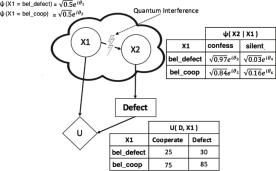
In this work, considering P r(πa) the classical probability distribution of the factor μ (X2, A) and f (πa) the classical utility corresponding to the choice of some action A of the same factor μ (X2, A), then we obtain

P r(πa) = P r (X1 = t) P r (X2|X1 = t) + P r (X1 = f ) P r (X2|X1 = f )

f (πa) = U (X1 = t, A) + U (X1 = f, A)

We can get the attraction factor, q(πa), by replacing the classical real numbers in P r(πa) by quantum-like amplitudes. The quantum interference e ects emerge by applying Born’s rule,

q(πa) = |ψ(X1 = t)ψ(X2|X1 = t) + ψ(X1 = f )ψ(X2|X1 = f )|2

q(πa) = |ψ(X1 = t)ψ(X2|X1 = t)|2 + |ψ(X1 = f )ψ(X2|X1 = f )|2 + 2Interf,

(17)

where the quantum interference term is given by

Interf = |ψ(X1 = t)ψ(X2|X1 = t)| |ψ(X1 = f )ψ(X2|X1 = f )| cos (θ1 − θ2) .

(18) Since the factor μ (X2, A) represented a probability distribution over the utility functions, we need to update the utility factor f (πa) in order to also represent this distribution over the quantum interference term. The quantum

interference term, for N random variables grows (Moreira and Wichert 2016)

N −1 N

2 |ψ(Xi = t)ψ(Xj |Xi = t)| |ψ(Xi = f )ψ(Xj |Xi = f )| cos (θi − θj ) .

i=1 j=i+1

The utility factor μ (X2, A) already specifies the utility function expressed in terms of the distribution of X2. When we consider X2 a quantum random variable, then this probability distribution is extended to incorporate the quantum

interference e ects. So, given that the utility function is expressed in terms of this probability distribution, we propose to update it in the same way as the interference term as

N

U (Xi = t, A) U (Xi = f, A) .

i=1

For our example, where we have utility factor μ (X2, A) expressed in terms of the distribution of X2, then

f (πa) = U (X1 = t, A) + U (X1 = f, A) + U (X1 = t, A) U (X1 = f, A) .

Under this representation, the result of the marginalisation, μ (X2, A), will be given by the product of the vector representation of the utility factor f (πa) with the attraction factor q(πa):

μ (X2, A) = q(πa)|f (πa) ,

where the vector representation corresponds to

This way, the final marginalisation for the quantum-like influence diagram is

μ (X2, A) = q(πa)|f (πa) = |ψ(X1 = t)ψ(X2|X1 = t)|2 · U (X1 = t, A) +

|ψ(X1 = f )ψ(X2|X1 = f )|2 · U (X1 = f, A) + Interf

, (19)

where

Interf = 2 |ψ(X1 = t)ψ(X2|X1 = t)| |ψ(X1 = f )ψ(X2|X1 = f )| cos (θ1 − θ2) .

Note that, in Eq. 20, if one sets the interference term (θi − θj ) to π/2, then cos(θi − θj ) = 0. This means that the quantum interference term is canceled and the quantum-like influence diagram collapses to its classical counterpart.

Finally, the goal is to find the decision rule δA that maximizes μ (X2, A),

We will refer to Eq. 20 as the quantum-like influence Equation, since we cannot call it a maximization of the expected utility in the real sense, because we had to change the distribution of the utility factor μ (X2, A) in order to mach the distribution over the quantum interference terms.

102 C. Moreira and A. Wichert

7A Quantum-Like Influence Diagram for the Prisoner’s Dilemma Game

Several paradoxical findings have been reported over the literature showing that individuals do not act rationally in decision scenarios under uncertainty (Kuhberger et al. 2001; Tversky and Shafir 1992; Lambdin and Burdsal 2007; Hristova and Grinberg 2008; Busemeyer et al. 2006a). The quantum-like influence diagram can help to accommodate the several paradoxical decisions by manipulating the quantum interference e ects that emerge from the inferences in the quantum-like Bayesian network, which can be used to reestimate the expected utilities.

Fig. 3. Quantum-Like Influence Diagram representing the Prisoner’s DIlemma Experiment from (Shafir and Tversky 1992). Random variable X1 corresponds to the player’s own believes about the action of his opponent (either believes the opponent will defect or the opponent will cooperate) and X2 corresponds to the player’s own strategy, i.e. either he confesses the crime or he remains silent.

We will model the works reported in Table 1 under the proposed quantumlike influence diagram. Figure 3 corresponds to the representation of the work of Shafir and Tversky (1992). The three types of nodes in the represented quantum-like influence diagram are the following:

–Random Variables: the circle-shaped nodes are the random variables belonging to the quantum-like Bayesian Network representing the player that needs to make a decision in the Prisoner’s Dilemma, without being aware of the decision of his opponent. We modelled this network with two binary random variables, X1 and X2. X1 corresponds to the player’s own believes about the action of his opponent (either believes the opponent will defect or the opponent will cooperate) and X2 corresponds to the player’s own strategy, i.e. either he confesses the crime (and therefore would find it safe to engage in a def ect strategy) or he remains silent (and would prefer to engage in a cooperate strategy). The tables next to each random variable are conditional probability tables and they show the probability distribution of the

variable towards its parent nodes. These conditional probability tables match the probability distributions reported in Table 1. In the specific case of Fig. 3, this table is filled with the values of the probability amplitudes identified in the work of Shafir and Tversky (1992).

–Action Node: the rectangle shaped node is the action that we want to make a decision. In the context of the prisoner’s dilemma we are interested to compute the maximum expected utility of defecting or not defecting (i.e. cooperating).

–Utility Node: the diamond shaped node corresponds to the payo s that the player will have for taking (or not) the action def ect, given his own personal strategy. The values in this node will be populated with the di erent payo s used across the di erent experiments of the prisoner’s dilemma game reported over the literature.

In the conditions where the player knows the strategy of his opponent, the quantum-like influence diagram collapses to its classical counterpart, since there is no uncertainty. This was already noticed in the previous works of Moreira and Wichert (2014, 2016, 2017). However, when the player is not informed about his opponent’s decision, then the quantum-like Bayesian network will produce interference e ects (Eq. 5). When computing the maximum expected utility, we will marginalise out X1 like it was shown in Eq. 16. This will result in a factor showing the distribution of the player’s personal strategy (either confess or remain silent) towards his believes over his opponents actions (either to defect or cooperate). The quantum interference term will play an important role to determine which quantum parameters can influence the player’s decision to switch from a classical (and rational) defect action towards the paradoxical decision found in the works the literature, i.e. to cooperate.

Fig. 4. Impact of quantum interference terms in the overall expected utility: (left) quantum parameters that maximize a cooperate decision, (center) variation of the expected utility when the player confesses (defects) and (right) variation of the expected utility when the player remains silent (cooperates).

Figure 4 demonstrates the impact of the quantum interference e ects in the player’s decision. The graphs in the centre and in the right of Fig. 4 represent