Материал: искусственный интеллект

Внимание! Если размещение файла нарушает Ваши авторские права, то обязательно сообщите нам

suai.ru/our-contacts

quantum machine learning

94 C. Moreira and A. Wichert

showing violations to the laws of classical probability and to the Sure Thing Principle. Table 1 summarises the results of several works of the literature reporting violations to the Sure Thing Principle. All of these works tested three conditions in the Prisoners Dilemma Game: (1) the player knows the other defected (Known to Defect), (2) the player knows the other cooperated (Known to Collaborate),

(3) the player does not know the other player’s action (Unknown). This last condition shows a deviation from the classical probability theory, suggesting that there is a significant percentage of players who are not acting according to the maximum expected utility hypothesis. The Sure Thing Principle (Savage 1954) principle is fundamental in the Bayesian probability theory and states that if one prefers action A over B under state of the world X, and if one also prefers A over B under the complementary state of the world X, then one should always prefer action A over B even when the state of the world is unspecified. Violations of the Sure Thing Principle imply violations of the classical law of total probability.

Table 1. Works of the literature reporting the probability of a player choosing to defect under several conditions. The entries of the table that are highlighted correspond to experiments where the violations of the sure thing principle were not found.

Literature

Known to

Known to

Unknown

Classical


defect

collaborate


probability


Shafir and Tversky (1992)

0.9700

0.8400

0.6300

0.9050


Li and Taplin (2002) (Average)

0.8200

0.7700

0.7200

0.7950


Li and Taplin (2002) Game 1

0.7333

0.6670

0.6000

0.7000


Li and Taplin (2002) Game 2

0.8000

0.7667

0.6300

0.7833


Li and Taplin (2002) Game 3

0.9000

0.8667

0.8667

0.8834


Li and Taplin (2002) Game 4

0.8333

0.8000

0.7000

0.8167


Li and Taplin (2002) Game 5

0.8333

0.7333

0.7000

0.7833


Li and Taplin (2002) Game 6

0.7667

0.8333

0.8000

0.8000


Li and Taplin (2002) Game 7

0.8667

0.7333

0.7667

0.8000


Table 1 presents several examples where the principle of maximum expected utility is not, in general, an adequate descriptive model of human behaviour. In fact, people are often irrational, in the sense that their choices do not satisfy the principe of maximum expected utility relative to any utility function (Koller and Friedman 2009).

Previous works in the literature have proposed quantum-like probabilistic models that try to accommodate these paradoxical scenarios and violations to the Sure Thing Principle (Busemeyer et al. 2006b, 2009; Pothos and Busemeyer 2009; Busemeyer and Bruza 2012). There is also a vast amount of work in trying to extend the expected utility hypothesis to a quantum-like versions Mura (2009); Yukalov and Sornette (2015). However, the expected utility framework alone poses some di culties, since it is very challenging the task of decision-making

suai.ru/our-contacts

quantum machine learning

Introducing Quantum-Like Influence Diagrams for Violations

95

in situations where the outcomes of an action are not fully determined (Koller and Friedman 2009).

In this paper, we try to fill this gap by taking into account the quantum-like probability inferences produced by a quantum-like Bayesian network to various outcomes and extend these probabilities to influence the preferences of an individual between these outcomes. Note that the probabilistic inferences produced by the quantum-like Bayesian network will su er quantum interference e ects in decision scenarios under uncertainty. The general idea is to use these quantum interference e ects to influence the expected utility framework in order to favour other actions than what would be predicted from the classical theory alone. We will combine this structure in a directed and acyclic compact probabilistic graphical model for decision-making, which we will define as the quantum-like influence diagram.

3A Quantum-Like Influence Diagram for Decision-Making

A Quantum-Like Influence Diagram is a compact directed acyclical graphical representation of a decision scenario, which was originally proposed by Howard and Matheson (1984). It consists on a set of random variables X1, . . . , XN belonging to a quantum-like Bayesian network. Each random variable Xi is associated with a conditional probability distribution (CPD) table, which describes the distribution of quantum probability amplitudes of the random variable Xi with respect to its parent nodes, ψ(Xi|P aXi ). Note that the di erence between a quantum-like Bayesian network and a classical network is simply the usage of complex numbers instead of classical real numbers. The usage of complex numbers will enable the emergence of quantum interference e ects. The influence diagram also consists in an utility node defined variable U , which is associated with a deterministic function U (P aU ). The goal is to make a decision, which maximises the expected utility function by taking into account probabilistic inferences performed on the quantum-like Bayesian network.

Fig. 2. General example of a Quantum-Like Influence Diagram comprised of a Quantum-Like Bayesian Network, X1, ..., XN , a Decision Node, D, and an Utility node with no children, U .

suai.ru/our-contacts

quantum machine learning

96 C. Moreira and A. Wichert

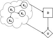
An example of a quantum-like influence diagram is presented in Fig. 2. One can notice the three di erent types of nodes: (1) random variable nodes (circleshape), denoted by X1, · · · , XN , of some Quantum-Like Bayesian Network, (2) a decision node (rectangle-shape), denoted by D, which corresponds to the decision that we want to make, and (3) an Utility node (diamond-shape), denoted by U , which in the scope of this paper, will represent the payo s in the Prisoner’s Dilemma Game.

The goal is to maximise the expected utility by taking into consideration the probabilistic inferences of the quantum-like Bayesian Network, which makes use of the quantum interference e ects to accommodate and predict violations to the Sure Thing Principle.

In the next sections, we will address each of these three components separately.

4 Quantum-Like Bayesian Networks

Quantum-like Bayesian Network have been initially proposed by Moreira and Wichert (2014, 2016) and they can be defined by a directed acyclic graph structure in which each node represents a di erent quantum random variable and each edge represents a direct influence from the source node to the target node. The graph can represent independence relationships between variables, and each node is associated with a conditional probability table that specifies a distribution of quantum complex probability amplitudes over the values of a node given each possible joint assignment of values of its parents. In other words, a quantum-like Bayesian Network is defined in the same way as classical network with the di erence that real probability values are replaced by complex probability amplitudes.

In order to perform exact inferences in a quantum-like Bayesian network, one needs to compute the:

Quantum-Like full join probability distribution. The quantum-like full joint complex probability amplitude distribution over a set of N random variables ψ(X1, X2, ..., XN ) corresponds to the probability distribution assigned to all of these random variables occurring together in a Hilbert space. Then, the full joint complex probability amplitude distribution of a quantum-like Bayesian Network is given by:

N


ψ(X1, . . . , XN ) = ψ(Xj |P arents(Xj ))

(2)

j=1


Note that, in Eq. 2, Xi is the list of random variables (or nodes of the network), P arents(Xi) corresponds to all parent nodes of Xi and ψ (Xi) is the complex probability amplitude associated with the random variable Xi. The probability value is extracted by applying Born’s rule, that is, by making the squared magnitude of the joint probability amplitude, ψ (X1, . . . , XN ):

P r(X1, . . . , XN ) = (X1, . . . , XN )|2

(3)

suai.ru/our-contacts

quantum machine learning

Introducing Quantum-Like Influence Diagrams for Violations

97

Quantum-Like Marginalization. Given a query random variable X and let Y be the unobserved variables in the network, the marginal distribution of X is simply the amplitude probability distribution of X averaging over the

information about Y . The quantum-like marginal probability can be defined by Eq. 4. The summation is over all possible y, i.e., all possible combinations of values of the unobserved values y of variable Y . The term γ corresponds to a normalisation factor. Since the conditional probability tables used in Bayesian Networks are not unitary operators with the constraint of double stochasticity (like it is required in other works of the literature (Busemeyer et al. 2006b; Pothos and Busemeyer 2009)), we need to normalise the final scores. This normalisation is consistent with the notion of normalisation of wave functions used in Feynman’s Path Diagrams.

In classical Bayesian inference, on the other hand, normalisation is performed due to the independence assumptions made in Bayes rule.


N


2


P r(X|e) = γ


ψ(Xk |P arents(Xk ), e, y)

(4)


y

k=1


Expanding Eq. 4, it will lead to the quantum marginalisation formula (Moreira and Wichert 2014), which is composed by two parts: one representing the classical probability and the other representing the quantum interference term (which corresponds to the emergence of destructive / constructive interference e ects):


|Y |

N

2


ψ(Xk |P arents(Xk ), e, y = i) + 2 · I nterf erence (5)

P r(X|e) = γ


i=1

k


I nterf erence =


|Y |−1

|Y |

N


N

i=1

j=i+1

ψ(Xk |P arents(Xk ), e, y = i) · ψ(Xk |P arents(Xk ), e, y = j) · cos(θi − θj )

k


k

Note that, in Eq. 5, if one sets (θi − θj ) to π/2, then cos(θi − θj ) = 0. This means that the quantum interference term is canceled and the quantum-like Bayesian Network collapses to its classical counterpart.

Formal methods to assign values to quantum interference terms are still an open research question, however some work has already been done towards that direction (Yukalov and Sornette 2011; Moreira and Wichert 2016, 2017).

5Maximum Expected Utility in Classical Influence Diagrams

In a decision scenario, D, given a set of possible decision rules, δA, the goal of Influence Diagrams is to compute the decision rule that leads to the Maximum Expected Utility. Additionally, P rδA (x|a) corresponds to a full joint probability

suai.ru/our-contacts

quantum machine learning

98 C. Moreira and A. Wichert

distribution of all possible outcomes, x, given di erent actions a belonging to the decision rules δA.

EU [D [δA]] = P rδA (x|a) U (x, a)

(6)

x


The goal is to choose some action a that maximises the expected utility with respect to some decision rule, δA:

a = argmaxδA EU [D [δA]]

One can map the expected utility formalism to the scope of Bayesian networks in the following way. Knowing that P rδA (x|a) corresponds to a full joint probability distribution of all possible outcomes, x, given di erent actions a belonging to the decision rules δA, this means that we can decompose the full joint probability distribution to the chain rule of probability theory as the product of each node with its parent nodes.

EU [D [δA]] =

P rδA (x|a) U (x, a)

(7)


x


EU [D [δA]] =

P r (Xi|P aXi ) U (P aU ) δA (A|Z)

(8)

X1,...,Xn ,A

i


In Eq. 8, Z = P aA represents the parent nodes of action A. We can factorise Eq. 8 in terms of the decision rule, δA, obtaining

EU [D [δA]] = δA (A|Z)

P r (Xi|P aXi ) U (P aU ) , (9)

Z,A

W i

where W = {X1, . . . , XN } − Z corresponds to all nodes of the Bayesian Network that are not contained in the set of nodes in Z.

By marginalising the summation over W , we obtain an expected utility formula that is written only in terms of the factor μ(A, Z). Note that this factor corresponds to a conditional distribution table of random variable Z (the outcomes of some action a) and action a.

EU [D [δA]] = δA (A|Z) μ (A, Z)

(10)

Z,A


The Maximum Expected Utility for a classical Influence Diagrams is given by (Koller and Friedman 2009):

δA

(a, Z) = α(x) =

1

a = argmax (A, Z)

(11)

0

otherwise