Материал: 4

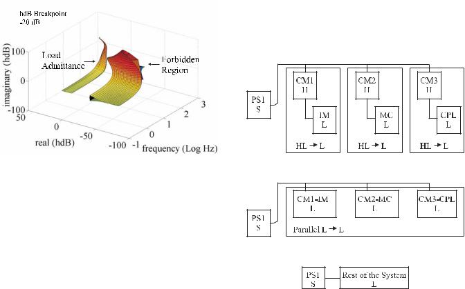
admittance. The forbidden region is obtained using the stability criteria as well as the generalized source impedance. The volume to the left represents a generalized load admittance.

Figure 9. Generalized load admittance and forbidden region for Case 1.

The basic ideas of generalized immittance analysis are set forth in [11], [12], and [13]. These papers primarily concern with simple source-load systems. The extension of the method to large-scale systems is considered in [14]. The first step necessary is to classify the power converters. Single-port converters are classified as S-converters (this category is normally for sources) or L-converters (this category is normally for loads). Two-port converters are classified as H-converters (normally for converters which accept power at one port and supply power to a second port), Y-converters (which are often loads fed by two busses), Z-converters (sources that have two outputs ) and C-converter (which are often cables). Formal definitions are set forth in [14]. Once all converters are classified, a series of mapping functions is used to reduce any given system to a source load equivalent. Many possible mapping operations are described in [14]. Often, these mapping operations involve a stability test to ensure that the aggregation of a subset of components is stable.

The steps to analyze the system are illustrated in Figure 10. Figure 10a depicts the original system for Case 1. In this case, CM4, CM5, CM6, and PS are removed from the system because for this scenario the starboard bus is out of service. Consideration of each of the components reveals that PS1 should be classified as an S-converter, CM1, CM2, and CM3 as H-converters, and the IM, MC, and CPL as L-converters. As indicated in Figure 10a, the first operation is three HL-L mappings that result in three aggregate L-converters – CM1-IM, CM2-MC, and CM3CPL. It should be noted that each of these mappings involves a stability test. In particular, for this mapping to be valid it has to be shown that if CM1 is fed from an ideal source then the system consisting of CM1 and IM is stable.

This is done by considering CM1 as a source and IM as a load [14]. The results of this test are not shown due to a lack of space. However, all zones pass this test for all the test cases described in Section 3. The next step is to aggregate the three effective L-converters with a parallel L to L converter mapping as shown in Figure 10b. This results in the system shown in Figure 10c, which consists of a single source and a single effective load. Details on converter types, mapping operations, and an example analysis of other system are set forth in [14].

(a). Original System.

(b). System after simplification.

(c). Final system.

Figure 10. Analysis steps.

Figure 9 depicts the final part of the stability analysis which considers the system of Figure 10c for Case 1. Again, the x-axis is log of frequency, the y-axis is real part of admittance in hybrid dB, and the z-axis is the imaginary part of admittance in hybrid dB. The volume to the right represents a forbidden region for the total system load admittance. The volume to the left represents the generalized load admittance (i.e. set of all possible values of load admittance). As can be seen, the generalized load admittance does not intersect the forbidden region. Thus, local stability (of at least the system model) is guaranteed for all operating points of interest. This is consistent with the results from the time-domain simulations.

Figure 11 depicts the results for Case 2. As can be seen, the generalized load admittance intersects the forbidden region. This does not mean that the actual system is unstable. However, there is no guarantee that the system is stable. From Figure 5 and Figure 6, it is seen that the system model is unstable.

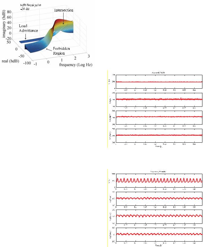
Figure 11. Generalized load admittance and forbidden region for Case 2.

6. EXPERIMENTAL VALIDATION

One of the key measures in evaluating these methods is how well they predict measured performance. Figure 12 and Figure 13 depict the measured time domain performance for Case 1 and Case 2 conditions, respectively. As can seen, all the stability methods consider thus far gave predictions consistent with the observed stability of the system.

7. POLYTOPIC ANALYSIS

In the preceding section, stability analysis of a power electronics based distribution system using time domain simulation and generalized immittance analyses were demonstrated, with excellent results. However, there are shortcomings inherent to either method. In the case of time domain simulation, the results are limited to a very narrow range of conditions. Massive numbers of trajectories must be evaluated to gain confidence in the system performance. In the case of generalized immittance analysis, in some sense a more powerful result is obtained. Using a single analysis, an entire range of operating points can be proven to be locally stable. Furthermore, this approach can be used as a design synthesis tool by providing a method to formulate component specifications. However, the generalized immittance design approach does not guarantee a bounded response in the presence of large disturbances. Hence, there is motivation to perform a stability analysis in which a system can be proven to have an appropriately bounded response to large disturbances.

To this end consider a broad class of nonlinear systems modeled by

are considered, where x n is the state vector, u m

is the input vector, and y p is the output vector. The

above nonlinear model is referred to as the truth model of the underlying system. Systems of this form may be analyzed by the direct method of Lyapunov [5] and [6]. However, there are difficulties associated with applying the direct method of Lyapunov including the determination of a valid Lyapunov function candidate [15]. Analytical means are often impractical if not impossible so a numerical approach is necessary. Through the use of polytopic modeling and linear matrix inequalities the search for possible Lyapunov function candidates can be automated.

Figure 12. Measured system performance for Case 1.

Figure 13 Measured system performance for Case 2.

7.2 Polytopic Models

Polytopic models are constructed combination of local models,

r

x& = ∑wi (θ)[Aix + Biu + i=1

y= wi (θ)[Cix + Diu + i=1r∑

Thus, (6) and (7) consist of r local models, defined by Ai,Bi,φxi,Ci,Di,φyi , combined by weighting functions,

wi . The weighting functions must satisfy 0 ≤ wi (θ) ≤ 1,

r

∑wi (θ) = 1, where θ may be a function of x or u .

i=1

Polytopic models can accurately represent the nonlinear system over a wide range of operation. Although the truth model already has this property the structure of the

8. POLYTOPIC ANALYSIS EXAMPLE

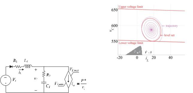
Consider the second order nonlinear system depicted in Figure 14 and having the parameters listed in Table 5. The source can be viewed as the NLAM of a 3-phase rectifier connected to an infinite bus [4]. The load can be viewed as the NLAM of a converter with a tightly regulated output and a valid operating range limited by the input voltage v1 , [18].

The states of this system are chosen as the inductor current, iL , and the capacitor voltage, vC . Local models

are obtained using Taylor series approximation at all combinations of 2.5A < iL < 50A , divided into 19 equally

spaced points, and 550V < v1 < 650V , divided into 20

equally spaced points. The local models are then forced to have coincident equilibrium pairs using the procedure given in the local modeling section. Using linear matrix inequalities (9) formed using the local models a common P is found,

that is symmetric and positive definite. This proves that the polytopic model is GUAS ISL.

Figure 14. Second order nonlinear system.

Table 5. Second order nonlinear system parameters.

To analyze the stability of the truth model, (11) is evaluated over a region of the state space surrounding the equilibrium state, see Figure 15. The region in which

V& > 0 is shaded black and the operating voltage limits for

the load are included as lines. The level set of V satisfying all three constraints forms an ellipse and is included along with one trajectory of the truth model. The ellipse identifies a region of uniform asymptotic stability for the truth model. The trajectory demonstrates the conservative nature of the Lyapunov based analysis.

The previous stability analysis methods discussed in this paper, time domain simulation and generalized immittances, both offer insight into the stability of nonlinear systems. However, neither of the methods identify a region of asymptotic stability about an equilibrium point. Polytopic model structure allows for the automatic search of Lyapunov function candidates,

which may be used to search for regions of asymptotic stability as seen in Figure 15. Further research into local model development and the determination of the region of asymptotic stability for higher order systems is on going.

Figure 15. V& evaluated over the state space.

9. ACKNOWLEDGEMENT

The authors would like to thank the Navy for its support of their efforts. This work was conducted under NAVSEA contract N00024-02-NR-60427 “Naval Combat Survivability” and ONR contract N00014-02-1-0990 “Polytopic Model Based Stability Analysis and Genetic Design of Electric Warship Power Systems.”

REFERENCES

[1]Pekarek et. al., A Hardware Power Electronic-Based Distribution and Propulsion Testbed, Sixth IASTED International Multi-Conference On Power and Energy System, Marina del Rey, California, May 12-15, 2002.

[2]S.D. Sudhoff, S.D. Pekarek, B.T. Kuhn, S.F. Glover, J. Sauer, D.E. Delisle, Naval Combat Survivability Testbeds for Investigation of Issues in Shipboard Power Electronics Based Power and Propulsion Systems, Proceedings of the IEEE Power Engineering Society Summer Meeting, July 21-25, 2002,Chicago, Illinois.

[3]S.D. Pekarek et. al., Development of a Testbed for Design and Evaluation of Power Electronic Based Generation and Distribution System, SAE2002 Power Systems Conference, Coral Springs, Florida, October 29-31, 2002.

[4]P.C. Krause, O. Wasynczuk, & S.D. Sudhoff, Analysis of Electric Machinery, 2nd ed., John Wiley & Sons, Inc., New York, 2002.

[5]S.H. Żak, Systems and Control, Oxford University Press, New York, 2003.

[6]H.K. Khalil, Nonlinear Systems, 2nd ed., Prentice Hall, Upper Saddle River, New Jersey, 1996.

[7]www.ESAC.info

[8]S.D. Pekarek, S.D. Sudhoff, J.D. Sauer, D.E.Delisle, E.J. Zivi, “Overview of the Naval Combat