Материал: 4

1. INTRODUCTION

Power electronics based power distribution systems are becoming increasingly common, particularly for mobile applications such as aircraft, vehicles, and on future ships. One of the defining characteristics of power electronics based systems is that they facilitate a high degree of automation and nearly instantaneous reconfiguration capabilities. Many power converters also feature nearly perfect regulation of their output objectives. For example, a dc/dc converter module may maintain an essentially constant output voltage regardless of input disturbances. From the output perspective, this property is highly desirable. However, it has unfortunate consequences. In particular, since power electronic converters are very efficient, ideal regulation of the output makes the converter appear as a constant power load from its input side. As such, an increase in input voltage will cause a decrease in input current – and hence the incremental input resistance to such a converter is negative. Negative incremental input resistance is destabilizing – and can result in instability of the interconnected power system. As a result, the stability analysis of such systems is of paramount importance.

In this paper, different methods of analyzing the stability of power electronics based power distribution systems are reviewed and applied to the Naval Combat Survivability

DC Distribution System [1], [2], [3]. This hardware testbed consists of ten power converters in a zonal architecture often considered for future Navy ships. Methods of stability analysis are discussed, with special emphasis on time-domain simulation, generalized immittance analysis, and the direct method of Lyapunov. The predictions of the time-domain simulation and the generalized immittance analysis are compared with experimentally measured results. In particular, these two methods are shown to predict the stability (or lack thereof) of the hardware test system. This is the first time the generalized immittance analysis approach has been validated in hardware on a system wide basis. The paper concludes with a discussion of future directions of stability analysis of power electronics based systems using nonlinear methods with emphasis on the use of polytopic modeling techniques.

2. STABILITY DEFINITIONS

It is appropriate to begin this paper with definitions of an equilibrium point, an operating point, and of stability. Definitions for these concepts are readily applied to a mathematical model of a system, but are not as readily applied to the system itself since the notion of state variables breaks down when discussing physical systems. Furthermore, even in the case of the mathematical model of a power electronics based system, the state variables in

a model detailed enough to portray the switching action of the power semiconductors will never become constant. Thus when defining terms related to stability it is necessary to differentiate those definitions as applied to a system model from those as applied to the system.

Herein, when referring to a mathematical model, an equilibrium point is a point at which the derivatives of the state variables are zero. In the case of a model in which switching is represented, the equilibrium point is a point at which the fast or dynamic average of the derivatives of the state variables are zero [4]. An operating point is defined as an equilibrium point about which the system is being studied. If conditions are such that there is only one possible equilibrium point then these terms become synonymous. An operating point of the system model is said to be locally stable if, when perturbed from an operating point by a small amount, the system model returns to that operating point. An operating point of the system model is said to be globally stable if the operating point can be perturbed by any amount and still return to that operating point.

In regard to the physical system (as opposed to a mathematical model), an operating point is defined to be the fast average of the voltages and currents that would satisfy power flow requirements for some loading condition. A dc power system is said to be locally stable about an operating point if the system voltages and currents vary only at the forcing frequencies associated with the switching of the power semiconductors and that the average values of these variables is such that all power converters are operating properly. In other words, the system is said to be stable if, neglecting switching induced ripple, the voltages and currents are constant in the steadystate and the level of these voltages and currents is such that all converters are operating in their intended modes of operation. Although this definition is admittedly informal and imprecise, it is nevertheless useful – particularly when we are discussing the stability of the system and not a model of the system.

These comments with regard to stability are intended for informal discussion only. For a thorough and rigorous discussion, the reader is referred to [5] and [6].

3. SYSTEM DESCRIPTION

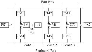
In order to illustrate the various methods of determining system stability, the Naval Combat Survivability DC Distribution Testbed depicted in Figure 1 is used as an example system. This reduced-scale hardware test bed was developed by the Navy and the Energy Systems Analysis Consortium (ESAC), (a consortium of universities) [7] in order to serve as a resource for researchers in Naval power and propulsion systems. It is intended to play a role analogous to the IEEE test systems for the electric utility grid.

Figure 1. Naval Combat Survivability DC Distribution

Testbed.

In this system, there are two power supplies (PS1 and PS2), one of which feeds the port bus, and the other of which feeds the starboard bus (only one connection is active at a time). There are three zones of dc distribution. Each zone is fed by a converter module (CM) on the port bus (CM1, CM2, or CM3) and a converter module on the starboard bus (CM4, CM4, or CM5) operating from one of the two distribution busses. Diodes prevent a fault from one bus being fed by the opposite bus. The converter modules feature a droop characteristic so that they share power. The three loads consist of an inverter module (IM) that in turn feeds an ac load bank (LB), a motor controller (MC), and a generic constant power load (CPL).

Robustness in this system is achieved as follows. First, in the event that either a power supply fails, or a distribution bus is lost, then the other bus will pick up full system load without interruption in service. Faults between the converter module and diode are mitigated by imposing current limits on the converter modules; and again the bus opposite the fault can supply the component. Finally, faults within the components are mitigated through the converter module controls. The result is a highly robust system.

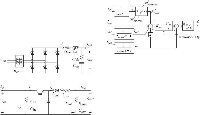
The discussion of the system components begins with the power supply. The power supplies PS1 and PS2 are identical, but have three operating modes. For the studies herein, the uncontrolled rectifier mode is considered. A schematic of the power supply in this mode is depicted in Figure 2. The primary side ac voltage is a nearly ideal 480 V l-l rms source at 60 Hz. The transformer parameters are: primary leakage inductance – 1.05 mH, primary winding resistance – 191 m Ω , secondary leakage inductance – 1.05 mH, secondary winding resistance - 191 m Ω , magnetizing inductance – 10.3 H, primary to secondary turns ratio 1.30. All of these parameters apply to the wye-equivalent T-equivalent transformer model and are referred to the primary winding. Finally, the dc link inductance, Ldc , is 9.93 mH, the resistance of this

inductance, rLdc , is 273 m Ω , the dc capacitor, Cdc , is 461

mF, and the effective series resistance of the dc capacitor, rCdc , is 70 m Ω . This capacitor is removed for some

studies as noted.

The circuit diagram for the converter modules is depicted in Figure 3. The parameters vary somewhat from converter module to converter module and are listed in Table 1.

Figure 2. Power supply.

Figure 3. Converter modules circuit diagram.

The control of the converter module is depicted in Figure 4. The principal variables not defined by Figure 3 and

Figure 4 are the commanded output voltage vout* and the commanded inductor current il* . This current command, in conjunction with the measured current il is used by a

hysteresis modulator so that the actual current closely tracks the measured current. The transfer function of the stabilizing feedback Hsf (s) is given by

Parameter values are listed in Table 2.

Figure 4. Converter module control.

Table 2. Converter Module Control Parameters.

Because of slight differences in the sensors combined with a fixed-point DSP, the integral voltage gain of the converters varies from converter to converter. The resulting value of Kiv for the six converter modules are (in

order): 220.6, 218.7, 216.4, 219.6, 219.7, and 218.7 A/Vs.

For the sake of brevity, the inverter module (IM), motor controller (MC), and constant power load (CPL) will not be discussed in detail herein. The salient dynamics of these components may be represented by a capacitor with capacitance Cx and effective series resistance rx in

parallel with an ideal constant power load of Px .

Parameters for this equivalent circuit are listed in Table 3. While this simplistic description can be used to a first approximation a more detailed analysis was used in the actual studies presented. The reader is referred to [1], [2], and [3] for a more detailed description of these components.

Table 3. Load Parameters.

Using this test system, two scenarios are studied. For each case, it is assumed that the starboard bus is out of service due to a fault and that the remainder of the system is being fed from the port power supply. All loads are operating at the capacity listed in Table 3. The difference between the two cases is the system parameters. For Case 1, all parameters are as listed thus far. For Case 2, the power supply output capacitance is removed, and the input capacitance to all the converter modules is reduced to the values listed in Table 4, and, in addition, the stabilizing filter gain, Ksf , of all the converter modules are set to

zero.

Table 4. Converter Module Parameters For Case 2.

4. TIME-DOMAIN SIMULATION

Perhaps the most straightforward means to examine system performance prior to experiment is through the use of time-domain simulation. There are fundamentally two types of simulations that are typically used in this class of systems – so-called ‘detailed’ model based simulations and non-linear average value model (NLAM) based simulations. The phrase ‘detailed’ is unfortunate because what is considered detailed is rather arbitrary. In terms of this discussion, however, ‘detailed’ refers to a simulation in which the switching action of each semiconductor is included, even if only on an ‘on’ or ‘off’ basis. Non-linear average value based models refer to simulations where the switching is represented on an average value basis. As a result, state variables are constant in the steady-state (Note that in ac systems, this is still true provided the model is expressed in a synchronous reference frame [4]).

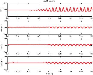
Figure 5 depicts the performance of the test system for the two cases described in the previous section. Variables depicted include:

Initially, the parameters are those for Case 1. As can be seen, the waveforms are constant, aside from the switching induced ripple. Approximately one-half of the way into the study, the parameters are changed to match Case 2. It should be observed that this change of parameters does not change the steady-state operating point. It is interesting to observe that the port bus voltage now contains a lowfrequency oscillation, which is not related to any of the

semiconductor switching frequencies. For this case, the system is predicted to be unstable.

Figure 5. Test system performance, detailed simulation.

In some sense, this study is unrealistic in that the parameters could not be physically changed in the prescribed way. The study is nevertheless useful in that it illustrates both stable and unstable systems with changes that do not affect the steady-state operating point.

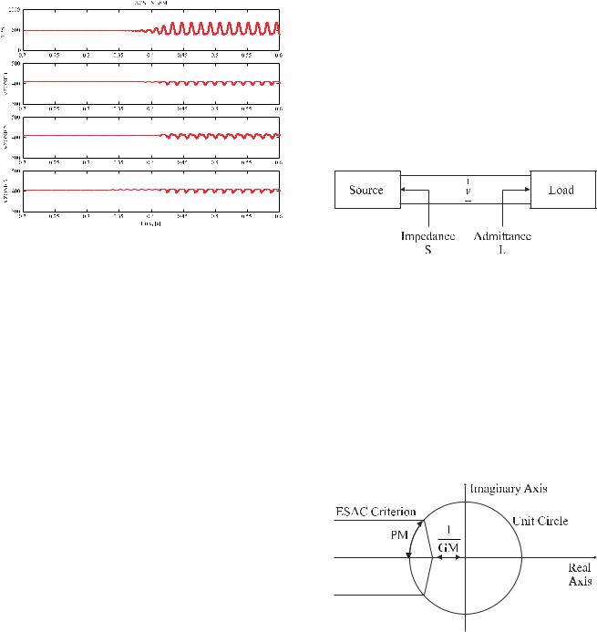
The waveforms shown in Figure 5 were obtained using a detailed model based simulation. Figure 6 depicts the waveforms using a NLAM based simulation. The first difference between Figure 5 and Figure 6 is the absence of the switching induced ripple in the waveforms. Otherwise, the simulations are compatible in their predictions, although the exact details of the waveforms vary once the instability has commenced. The reason for this is that models of unstable nonlinear systems tend to exhibit chaotic like behavior – they are extremely sensitive to small differences, for example, in parameters and modeling techniques. The observation that the two models agree well during transients involving stable conditions [8] supports this hypothesis.

Although the conclusions of each time-domain study are similar, there are significant differences between the two time-domain simulations. The NLAM has a computational advantage in that the dynamics are not periodically excited by the switching of the semiconductors. As a results, integration algorithms for stiff systems can be used more effectively than for detailed model simulations. For this system, simulating the 83rd order detailed system model for 0.7 s required 262.3 s of CPU time on a 1 GHz Pentium processor based machine. This time was obtained using the a 5th order Runge-Kutta-Fehlberg integration algorithm

with a maximum time step of 10−5 s, a minimum time step

of 10−11 s, and a data logging rate 10−4 s. The same study required 55.4 s on the same CPU using the 77th order

NLAM model. In this case Gear’s algorithm was used and all other parameters were the same except that the

minimum time step was 10−15 s.

Figure 6. Test system performance, NLAM simulation.

An additional feature of NLAMs is that they can be automatically linearized using many simulation languages including MATLAB [9] and ACSL [10].

As a tool for examining stability, however, the use of timedomain simulation has drawbacks. The primary drawback is that a given study only predicts the stability of a single operating point for a particular perturbation. One valid approach to gain confidence in system behavior is to run massive numbers of studies. However, there is always a possibility that an unstable operating point or scenario can be overlooked.

5.GENERALIZED IMMITTANCE ANALYSIS

For linear systems, the most straightforward alternative to using time domain simulation for examining system stability is to find and inspect the eigenvalues. However, this class of systems is non-linear thereby limiting the usefulness of linear system analysis. One approach can be to simply linearize the system about a given operating point, though such an approach would face the difficulty of needing to check each and every operating point of interest (and there may be infinitely many of them).

An alternative technique, which is also at its roots based in linear system theory is to use the method of generalized immittance analysis [11], [12], [13], and [14]. This is a frequency domain based technique, which has two important characteristics. First, in a single analysis it can be used to test the local stability of all operating points of interest. Second, unlike eigenanalysis, it can be used to set forth design specifications that ensure this condition. For

example, in a simple source load system, given a source the method can be used to deduce properties that the load must satisfy in order to ensure the local stability of all operating points of interest.

To illustrate this method, consider the simple source-load system of Figure 7. Let the small-signal impedance

characteristic of the load be denoted Yx . Let the set Z

represent the generalized impedance and the set Y represent the generalized admittance. Thus, Z x Z andYx Y for all operating points of interest. The

variation of values stems both from nonlinearities as well as parameter uncertainties.

Figure 7. Simple source – load system.

The next step is to select a stability criteria in the s-plane. Figure 8 depicts the ESAC stability criteria with a gain margin GM and phase margin PM. Using generalized admittance analysis, based on a generalized source impedance (load admittance) a load admittance (source impedance) constraint is found such that as long as the generalized load admittance (source impedance) does not intersect the forbidden region then the Nyquist contour of Z x Yx will not cross the stability criteria boundary. This

in turn ensures that the Nyquist contour of Z x Y x cannot

encircle –1, which in turn ensures that all operating points considered are locally stable.

Figure 8. ESAC stability criteria.

The constraint formed is best viewed in the immittance space. To this end, consider Figure 9. The x-axis of this figure is log of frequency, the y-axis is real part in hybrid dB [14], and the z-axis is imaginary part in hybrid dB. The volume to the right is a forbidden region to the load