Материал: искусственный интеллект
suai.ru/our-contacts |
quantum machine learning |
Weights in CQQL
Fig. 2 Equiangular mapping
|
135 |
|1 |
|
a = 7a = 6 |
|
a = 5 |
|
a = 4 |
|
a = 3 |
|
a = 2 |
|
a = 1 |
|
a = 0 |
|
1 |
|0 |
Ðdatabase condition: A traditional database condition returns just Boolean values. This can be simulated by mapping bijectively every possible attribute value to exactly one basis vector. These vectors are mutually orthonormal. Thus, querying values produces only two possible results, a 1 on match and a 0 on mismatch.
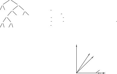
Ðproximity condition: The values for a proximity condition are encoded by vectors of different non-orthogonal angles. For example, Fig. 2 depicts the encoding of
eight values in a qubit. Following that encoding [2], the evaluation of a condition that requires an eight-value attribute c having the value b returns cos2 |a−c|π/16.
The starting point of CQQL conditions is a set of commutative conditions.
Definition 5 Let A |
= {aj } be a Þnite set of attributes and AC |
= |
{aci (aj )} |
|||||||||
be a Þnite set of |
atomic |
attribute |
conditions |
of |
the |
form |
Òa |
= |
valueÓ |
|||
|
2 |
|
j |
|||||||||
or proximity conditions of |
the |
form Òaj ≈ |
value.Ó |
|
Let furthermore be |
|||||||
given a function |
vs(aci (aj )) |
= |
1 |
ki |
} which |
assigns |
to every |
|||||
{aci , . . . , aci |
||||||||||||
condition a set of orthonormal vectors forming a vector subspace. The condition set AC is called commutative if aci1 (aj1 ), aci2 (aj2 ) AC :
type(aci1 (aj1 )) = d |
type(aci2 (aj2 )) = d j1 = j2 # i1 = i2 holds where |
type returns d for a |
database condition and p or r for a proximity or retrieval |
condition, respectively.
Commutativity means that no two proximity or retrieval conditions Òaj ≈ value1Ó and Òaj ≈ value2Ó with value1 = value2 on the same attribute aj are allowed.
Lemma 1 Let AC be a commutative set of atomic conditions over A = {aj }. The
set CV S(AC) = |
vs(aci (aj )) is a set of mutually orthonormal vectors. |
|
aci (aj ) AC |
The lemma is a direct consequence of how the mapping function vs is realized (for more details, see [2]). It is very essential because it means that every subset of CV S(AC) spans a vector subspace and corresponds bijectively to a CQQL condition.
2Without loss of generality and for simplicity we ignore here atomic conditions on more than one attribute, which are discussed in [2].
suai.ru/our-contacts |
quantum machine learning |
136 I. Schmitt
Definition 6 Let AC be a commutative set of atomic conditions on A = {aj }. Then a CQQL condition ϕ is recursively deÞned by
Ð |
|
def |
(aj ) AC |
ϕ = aci |
|||
Ð |
|
def |
ϕ2) |
ϕ |
= (ϕ1 |
||
Ð |
|
def |
ϕ2) |
ϕ |
= (ϕ1 |
||
def
Ðϕ = (¬ϕ1),
where ϕ1, ϕ2 are CQQL conditions.
Theorem 1 All CQQL conditions over a commutative set of atomic conditions together with conjunction, disjunction, and negation form a Boolean algebra.
Proof The function vs maps bijectively every condition to a subset of CV S(CS). Conjunction, disjunction, and negation are mapped to their corresponding set operations:
vs(aci (aj )) CV S(AC)
vs(ϕ1 ϕ2) = vs(ϕ1) ∩ vs(ϕ2) CV S(AC)
vs(ϕ1 ϕ2) = vs(ϕ1) vs(ϕ2) CV S(AC)
vs(¬ϕ1) = CV S(AC) \ vs(ϕ1) CV S(AC).
A set together with these standard set operations and the orthocomplement for the negation is a Boolean algebra. &%
The CQQL conjunction is also a valid t-norm and the disjunction a valid t-conorm. In contrast to known fuzzy norms, they fulÞll all Boolean algebra rules including distributivity, absorption, and idempotence. An interesting result from [2] is the fact that a complex CQQL condition in a speciÞc syntactical form can be evaluated by means of simple arithmetics.
Definition 7 Let the function att return for every condition the set of its restricted attributes. Following [2] we deÞne for an object o the evaluation f of a conjunction and disjunction of non-overlapping conditions as well of an exclusive disjunction. The negation is just the subtraction from 1.
fϕ1 ϕ2 (o) = "CQQL(fϕ1 (o), fϕ2 (o)) = fϕ1 (o) · fϕ2 (o) if att (ϕ1) ∩ att (ϕ2) = . fϕ1 ϕ2 (o) = CQQL(fϕ1 (o), fϕ2 (o))
= fϕ1 (o) + fϕ2 (o) − fϕ1 (o) · fϕ2 (o) if att (ϕ1) ∩ att (ϕ2) = . fϕ1 ϕ2 (o) = CQQL(fϕ1 (o), fϕ2 (o))
= fϕ1 (o) + fϕ2 (o) if ac : ϕ1 = Ôac φ1Ô ϕ2 = Ô(¬ac) φ2Ô f¬ϕ (o) = 1 − fϕ (o).
suai.ru/our-contacts |
quantum machine learning |
Weights in CQQL |
137 |
Since our language obeys the rules of a Boolean algebra we can transform every possible CQQL condition into the required syntactical form, e.g., the disjunctive normal form or the one-occurrence-form [8]. Schmitt [2] gives an algorithm performing this transformation.
Our example condition without weights is a CQQL condition being already in the required form. Following DeÞnition 7 we obtain svT (o) · svA(o) · (svD (o) + svS (o) − svD (o) · svS (o))(1 − svP (o)) for an object o to be evaluated.
5 Logic-Based Weighting
Our approach of weighting CQQL conditions is surprisingly simple. The idea is to transform a weighted conjunction or a weighted disjunction into a logical formula without weights:
|
w (ϕ1 |
,ϕ2) |
(ϕ1 |
¬ |
θ1) |
|
(ϕ2 |
¬ |
θ2) |
and |
w (ϕ1,ϕ2) |
(ϕ1 |
|
θ1) |
|
(ϕ2 |
|
θ2). |
|
|
θ1,θ2 |
# |
|
|
|
|
|
θ1,θ2 |
# |
|
|
|
|
||||||
Definition 8 |
Let o be a database object, svac(o) [0, 1] a score value obtained |
||||||||||||||||||
from evaluating an atomic CQQL condition ac on o, Θ = {θ1, . . . , θn} with θi [0, 1] a set of weights, and ϕ a CQQL condition constructed by recursively applying, , θi ,θj , θi ,θj , and ¬ on a commuting set of atomic conditions. The weighted score function is deÞned by
f Θ |
|
|
(o) |
(ϕ1¬θi ) (ϕ2¬θj ) |
|
||
f Θ |
|
(o) |
|
(ϕ1 θi ) (ϕ2 θj ) |
|
|
|
"CQQL |
fϕΘ1 (o), fϕΘ2 (o) |
||
fϕΘ (o) = CQQL |
fϕΘ1 (o), fϕΘ2 (o) |
||
1 − fϕΘ1 (o) svac(o) svacθ
if ϕ = ϕ1 θi ,θj ϕ2
if ϕ = ϕ1 θi ,θj ϕ2
if ϕ = ϕ1 ϕ2 if ϕ = ϕ1 ϕ2 if ϕ = ¬ϕ1
if ϕ = ac if ϕ = θ.
svacθ can be regarded as a special atomic condition without argument returning the constant θ .
Our weighting does not require a special weighting formula outside of the context of logic. Instead it uses exclusively the power of the underlying logic. Please notice that we can weight not only atomic conditions but also complex logical expressions. Thus, our approach supports a nested weighting.
Figure 3 (left) shows the result of applying our mapping rules onto the weighted tree from Fig. 1. Following our CQQL evaluation we obtain the formula
suai.ru/our-contacts |
quantum machine learning |
138 |
|
|
|
|
|
|
|
|
|
|
I. Schmitt |
|
|
|
|
|
|
|
|
|
|
|
|
|
|
|
|
|
|
|
|
|
|
|
|
|
|
|
|
|
|
|
|
|
name |
θD |
θS |
θDS |
θP |
winner |
|
T A |
|
|
|
|
|
equi weight |
1 |
1 |
1 |
1 |
fair |
|
|
|
|
nonrelevant price |
1 |
1 |
1 |
0.1 |
deluxe |
|
|||
|
¬ |
¬ |
|
¬ |
|
|
||||||
|
P |
θP |
very relevant price |
1 |
1 |
0 |
1 |
cheap |
|
|||
|
|
θDS |
|
|
||||||||
|
|
|
|
|
|
very relevant date |
1 |
0.4 |
1 |
0.2 |
exact date |
|
|
|
|
|
zero weight |
0 |
0 |
0 |
0 |
cheap |
|
||
|
|
|
|
|
|
|
||||||
D θD S |
θS |
|
|
|
|
|
|
|
|
|
|
|
Fig. 3 Expanded weighted condition tree and weight settings
Fig. 4 Weight mapping for θ = 1/4 and θ = 1/2
|1 |
w = π/3 for θ = 1/4 |
w = π/4 for θ = 1/2 |
vector for constant 1 |
1 |0 |
fϕΘ (o) = svT (o) · svA(o) · svDSθ (o) · sv¬P θP (o)
svDSθ (o) = svDS (o) + (1 − svθDS ) − svDS (o) · (1 − svθDS )
svDS (o) = svD (o) · svθD + svS (o) · svθS − svD (o) · svθD · svS (o) · svθS sv¬P θP (o) = (1 − svP (o)) + (1 − svθP ) − (1 − svP (o)) · (1 − svθP ).
The table in Fig. 3 (right) shows the chosen weight values and the corresponding cottages with the highest score value. Of course, for an end user it is not easy to Þnd the right weight values. Instead, we propose the usage of linguistic variables like very important, important, neutral, less important, and not important and map them to numerical weight values. Another possibility is to use graphical weight sliders to adjust the importance of a condition.
Next, we show that our weighting approach fulÞlls our requirements.
Theorem 2 The weight functions as defined in Definition 8 fulfill the requirements R1 to R5.
Proof Following Theorem 1, CQQL conditions with conjunction, disjunction, and negations form a Boolean algebra. Our approach uses special atomic conditions acθ for different weights θ (Fig. 4).
As demonstrated, our weighting is realized inside the CQQL logic. Thus, it is easy to show the fulÞllment of the requirements:
1.(R1) weight=0: w0",1(a, b) = (a ¬0) (b ¬1) = 1 b = b. The commutative variant and the disjunction are analogously fulÞlled.

suai.ru/our-contacts |
quantum machine learning |
Weights in CQQL |
139 |
2.(R2) weight=1: w1",1(a, b) = (a ¬1) (b ¬1) = a b = "CQQL(a, b)
(analogously for ).
3.(R3) continuity: The weight functions are continuous on the weights since the underlying squared cosine function, conjunction, and disjunction are continuous.
4.(R4) embedding in a logic: Since our weighting is realized inside the logic formalism the resulting logic is still a Boolean algebra. The proof of the four formulas is thus straightforward.
5.(R5) linearity: The evaluation of a weighted CQQL conjunction and disjunction w.r.t. one weight is based on linear formulas.
So far, we applied our weighting approach to retrieval and proximity conditions of our CQQL language. What about applying it exclusively to traditional database conditions returning just Boolean values? In that case, we distinguish between two cases:
1.Non-Boolean weights: If the weights come from the interval [0, 1], then we
cannot use the normal Boolean disjunction and conjunction. Instead we propose to replace them with the algebraic sum (x + y − x · y) and the algebraic product (x · y). This case can be regarded as a special case (only database conditions) of CQQL and it fulÞlls the requirements (R1) to (R5) if each condition is not weighted more than once. Otherwise we transform, see [2], that formula into
the required form. Table 2 shows the effect of non-Boolean weights on database conditions whose evaluations are expressed by x and y.
2. Boolean weights: If the weights are Boolean values, then we can evaluate a weighted formula by using Boolean conjunction and disjunction fulÞlling requirements (R1), (R2), and (R4). Requiring continuity (R3) and linearity (R5) on Boolean weights is meaningless. Boolean weights have the effect of a switch. A weighted condition can be switched to be active or inactive.
At the end, we present (x θ ) (y ¬θ ) as an interesting special case where one connected weight instead of two weights is used. In this case, the resulting evaluation formula is the weighted sum: θ svx (o) + (1 − θ ) svy (o). Very surprisingly, next logical transformation3 shows that connected weights of a conjunction equal exactly connected weights of a disjunction.
Table 2 Weights on Boolean conditions
x |
|
y |
|
|
x θ,1 y := x + |
|
|
|
|
x θ,1 y := θ x + y − θ xy |
||
|
|
θ |
− xθ |
y |
||||||||
0 |
(false) |
0 |
(false) |
0 |
(false) |
0 |
(false) |
|||||
0 |
(false) |
1 |
(true) |
|
|
|
|
|
|
|
1 |
(true) |
|
θ |
|
|
|
|
|
||||||
1 |
(true) |
0 |
(false) |
0 |
(false) |
θ |
|
|||||
1 |
(true) |
1 |
(true) |
1 |
(true) |
1 |
(true) |
|||||
3For a simple notation, conjunction is expressed by a multiplication and disjunction by an addition symbol.