Материал: Russian Journal of Building Construction and Architecture

Russian Journal of Building Construction and Architecture

used. Coupling of the reinforcement with concrete was investigated under varying loads and external conditions with a fixed shift of the upper 1 and lower ends of the reinforcement bar 2. The periodic reinforcement of two types was considered:

––a metal reinforcement А400 of steel 25Г2С with a fluidity area;

––a glass plastic reinforcement with no physical fluidity limit.

The strain distribution at the early stages of pulling was uneven but became almost homogeneous in the limiting state. Therefore the expression of the limiting coupling effort is seen as an average strain between concrete and reinforcement. This calculation method of τсц (equation (1)) provides a practical approach to identifying the coupling strength between concrete and reinforcement while it does not reflect the actual state of the structure as it does not account for such factors as cracking caused by strain, local bearing stress, support reaction, etc. Therefore τсц between reinforcement and concrete was calculated using the average tangential strain given by the equation (1):

where N is the targeted effort; l is the anchorage depth; Р is the perimeter of the circle.

The model used 6 critical parameters such as the compressive strength of the concrete prism, stretching strength of concrete, elasticity modulus of concrete, anchorage depth, profile and material of reinforcement. The strength characteristics were specified in accordance with the GOST (ГОСТ) 24452-80, the freezing and thawing cycles were conducted in accordance with the GOST (ГОСТ) 10060-2012.

These predictive parameters were employed in order to develop the model for evaluating the final compressive strength between reinforcement and concrete. Table 1 presents the ranges of each variable. In order to model the coupling properties the database was randomly divided into three parts: training, control and testing. 15 % of the experimental data was used for testing, another 15 % for control and the remaining 70 % for training the network. As a result of the control, the risk of having to train the network again was reduced. The training database was employed for developing the predicting model as the testing database was used for observing the pattern and reliability of the suggested models NN.

2. Artificial neural networks. Artificial neural networks (NN) were developed according to the principle of the operation of biological neural networks in the body and is a simplified mathematical model.

The principle of designing such a model was formulated by McCulloch and Pitts in 1943 where NN is a simplified model of biological neural networks. A system was obtained that

10

consists of simple (computational) mathematical blocks (neurons) connected with weighed bonds (synapsis). Due to being simple and universal, artificial neural networks are currently widely used in sciences including physics, medicine, technology, etc. Construction materials and mechanics is one of these.

In the early 1990s Т. Nitta developed a more advanced model NN which became widely used in engineering tasks. In the suggested model NN the parameters (threshold values, weight, input and output massives) are presented by complex numbers to enable it to be employed in different industries of modern technology such as data hierarchy, speech analysis, data collection, time analysis of neural systems, etc. Use of NN in construction is a newly emerging research field. This paper presents the results of the model based on NN in the MatlabV.R2014a environment using the nnstar tool.

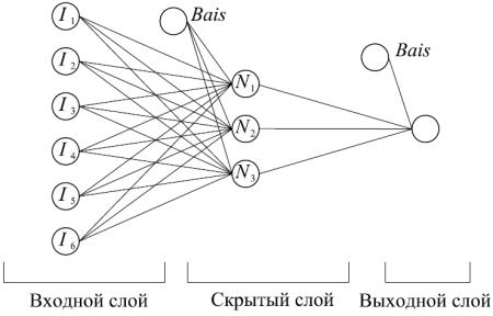
3. Architecture of the neural network and model in the clear form. The architecture of NN at the input level has six nodes corresponding with six predicting factors, three nodes in the hidden layer (N1––N3) and one in the output layer corresponding with the limit coupling strength τсц between reinforcement and concrete. Therefore in order to design the model using NN the architecture 6-3-1 of NN was obtained (Fig. 2).

Fig. 2. Аrchitecture of NN for the suggested model

The model NN used in the current study can be simply expressed with the equation (2). The details of the input and output layers, the function of activation (hyperbolic tangent) and bias are given in the equations (2)––(5). Note that all the numerical variables should be normalized

11

Russian Journal of Building Construction and Architecture

(I1 – I6) to the range [–1, 1] before being introduced into NN. It is thus necessary to introduce normalized values specified for the model NN into the mathematical procedures. It should also be noted that the final result obtained from the equation (3) should be normalized and denormalized according to the normalization coefficients a, b (Table 2) specified in [11].

Note: βmax, βmin is the maximum and minimum of the dataset.

In order to design the model for searching for the weighs of the network the LevenbergMarquardt algorithms LM were used:

j 1

where Biasoutput layer = 0.096779740634 is the shift in the neuron of the output layer; F(U) (hyperbolic tangent) is an activation function; g(U) is a denormalization function.

0.353067120271963 th(U2 ) 0.158184154640520 th(U3)),

where τсц is the final coupling strength between reinforcement and concrete, МPа; wk is the matrix weighs; th(U) is an activation function (hyperbolic tangent) given by the equation (4); U1, U2, ..., U3 can be calculated using the formula (5):

12

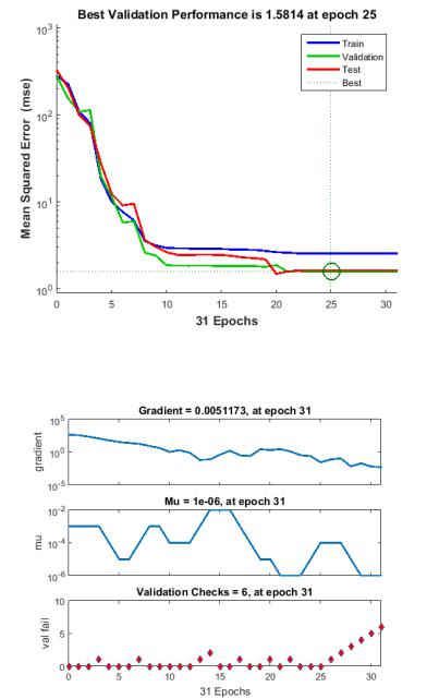
The training results of the network are presented in Fig. 3, the state of the artificial neural network during the training is in Fig. 4.

Fig. 3. Training results of the network

Fig. 4. State of the artificial neural network during the training

13

Russian Journal of Building Construction and Architecture

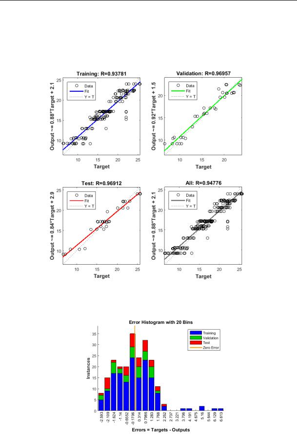
Comparison of the prediction results obtained using the model NN and experimental data obtained as a result of the coupling tests is shown in Fig. 5. The correlation coefficients 0.969 and 0.969 were reached for the control and training databases respectively.

Fig. 5. Regression analysis of the model

Fig. 6. Error histogram

14